


Preliminary steps
👉 This tutorial requires that you have installed node template Import images.
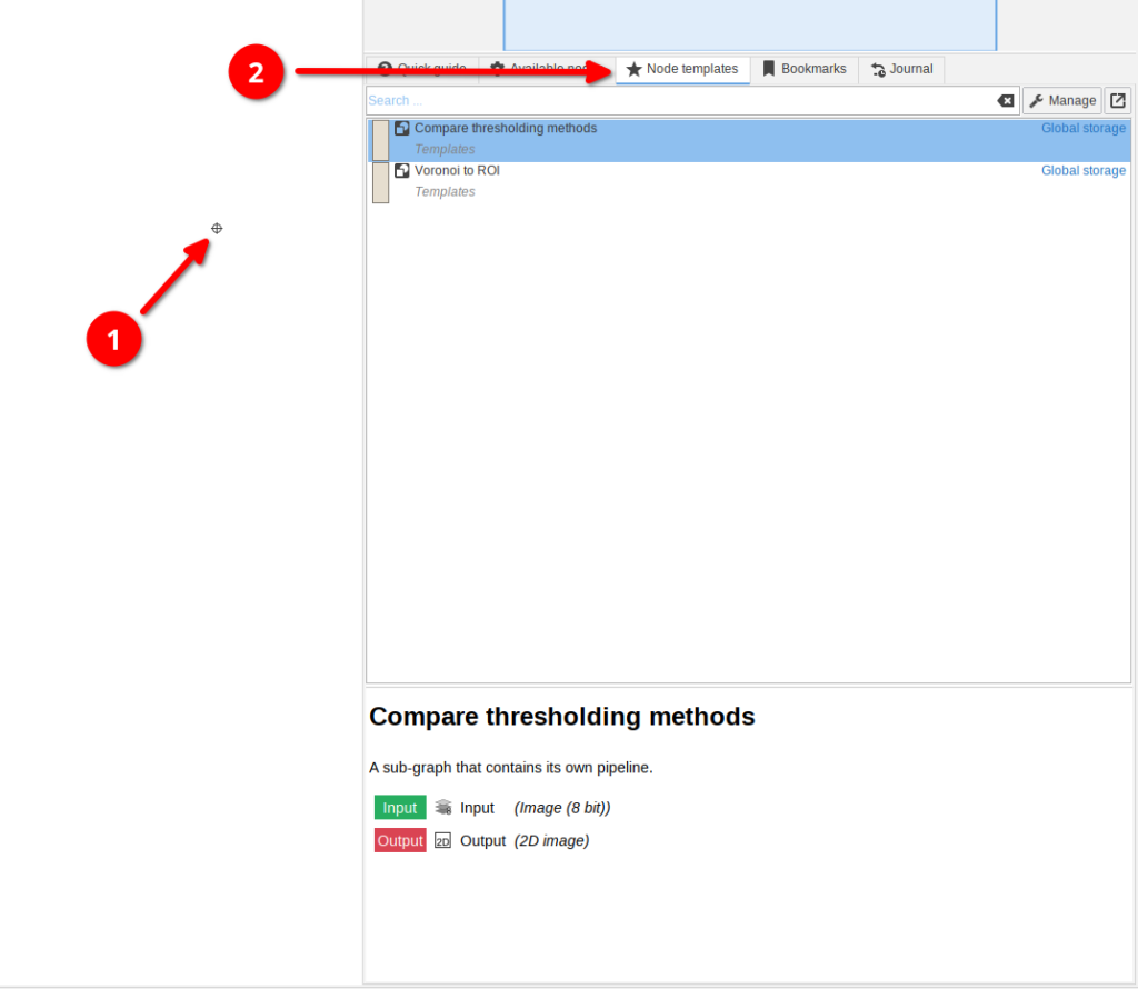
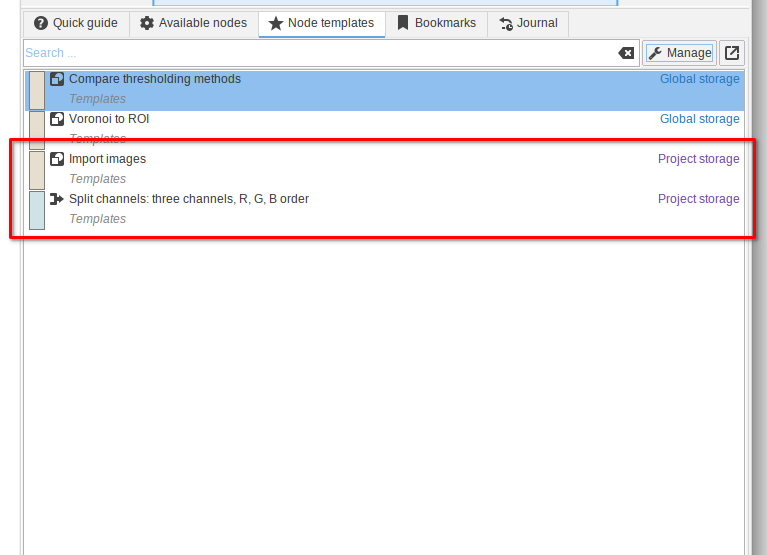
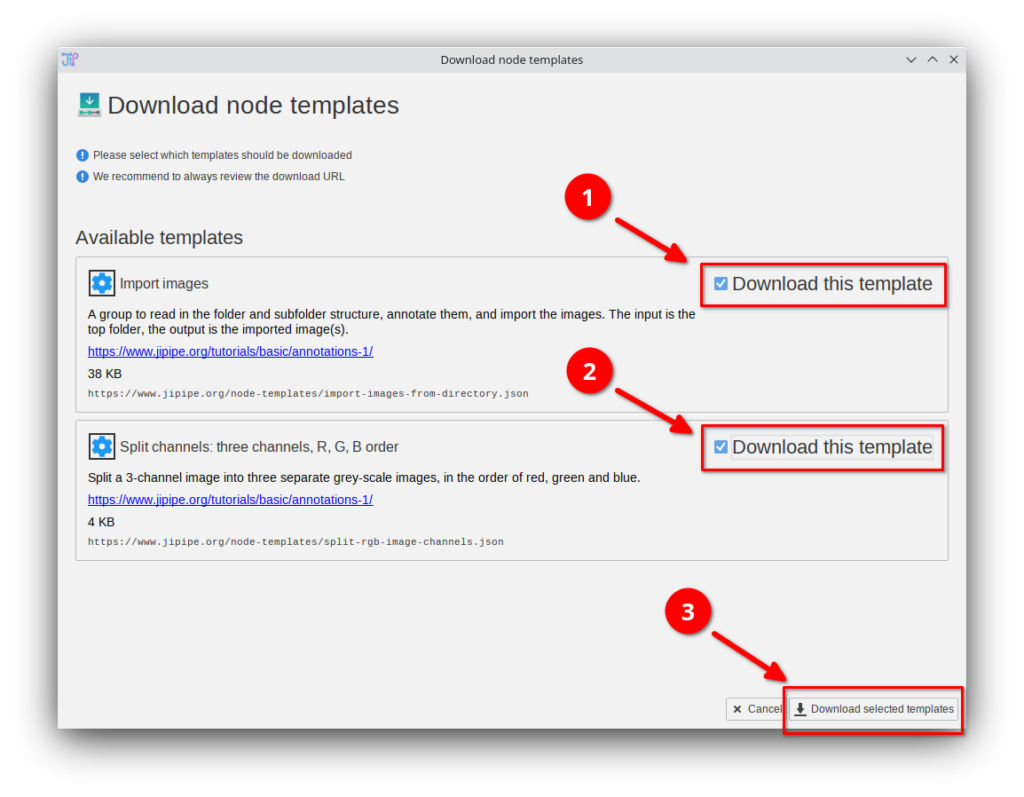
If you do not have these templates, you can download them via Manage > Download more templates or by importing the Templates.json file that is provided in the data package. If you do not know how to download or import node templates, please check out our tutorial.
Step 1
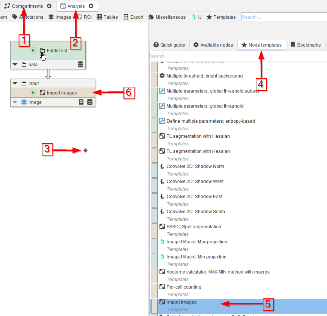
Create a new project from the one-compartment template (red arrow 1), open the Analysis compartment (red arrow 2).
Download and extract the data package for this tutorial and drag the data directory into the Analysis compartment.
Click anywhere in the white area of the UI (red arrow 3) and select the Node templates tab (red arrow 4).
Select the Import images group node (red arrow 5) and drag it to the UI (red arrow 6). Connect Folder list to the Import images input.
Step 2
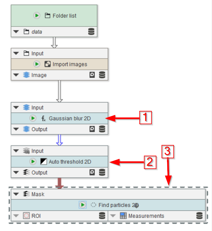
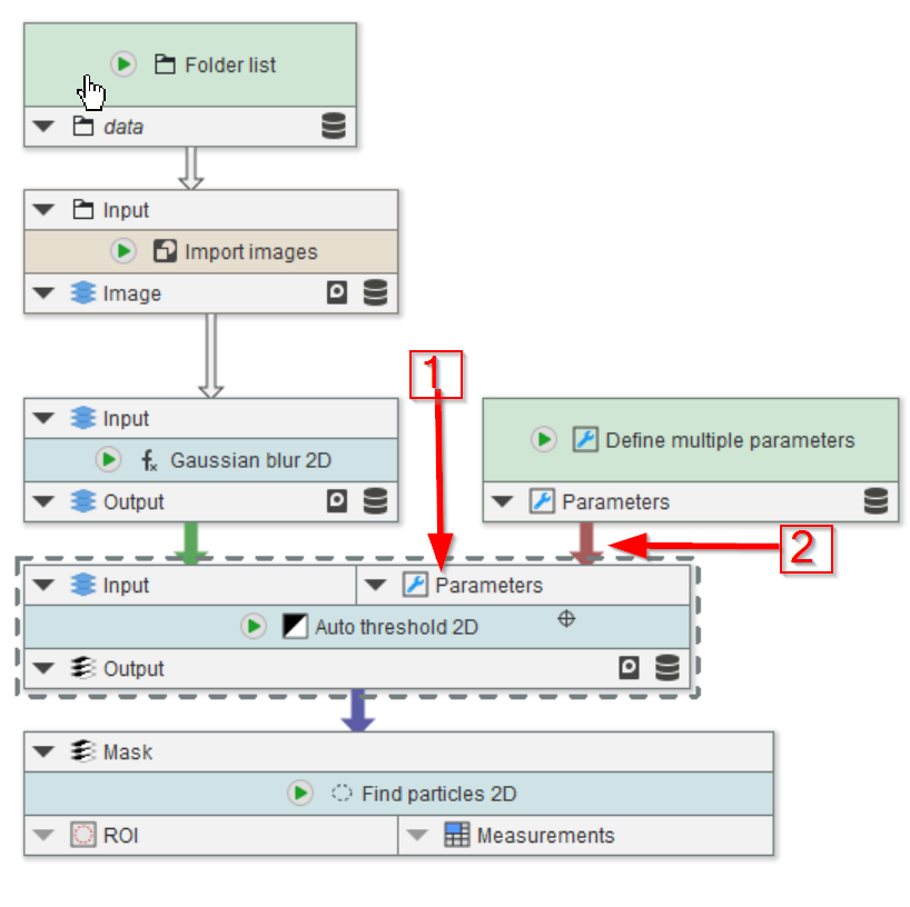
Add a Gaussian blur 2D (red arrow 1) and an Auto threshold 2D node (red arrow 2), as well as a Find particles 2D node (red arrow 3) to the UI and connect them as shown in the figure.
Step 3
Gaussian blurring and thresholding are both sensitive to their parameter settings.
Thus it is often useful to test multiple parameters for such nodes by connecting them up to a selection of parameters that can be tested within the same run of the project.
In JIPipe, multiple parameter sets are defined by a dedicated set of nodes, one of which is termed Define multiple parameters.
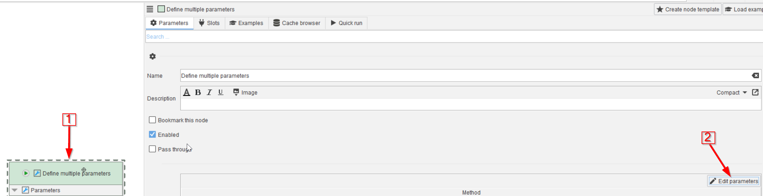
Begin by adding Define multiple parameters into the pipeline (red arrow 1). Select the node and click the Edit parameters option in the node Parameters tab (reds arrow 2).
Step 4
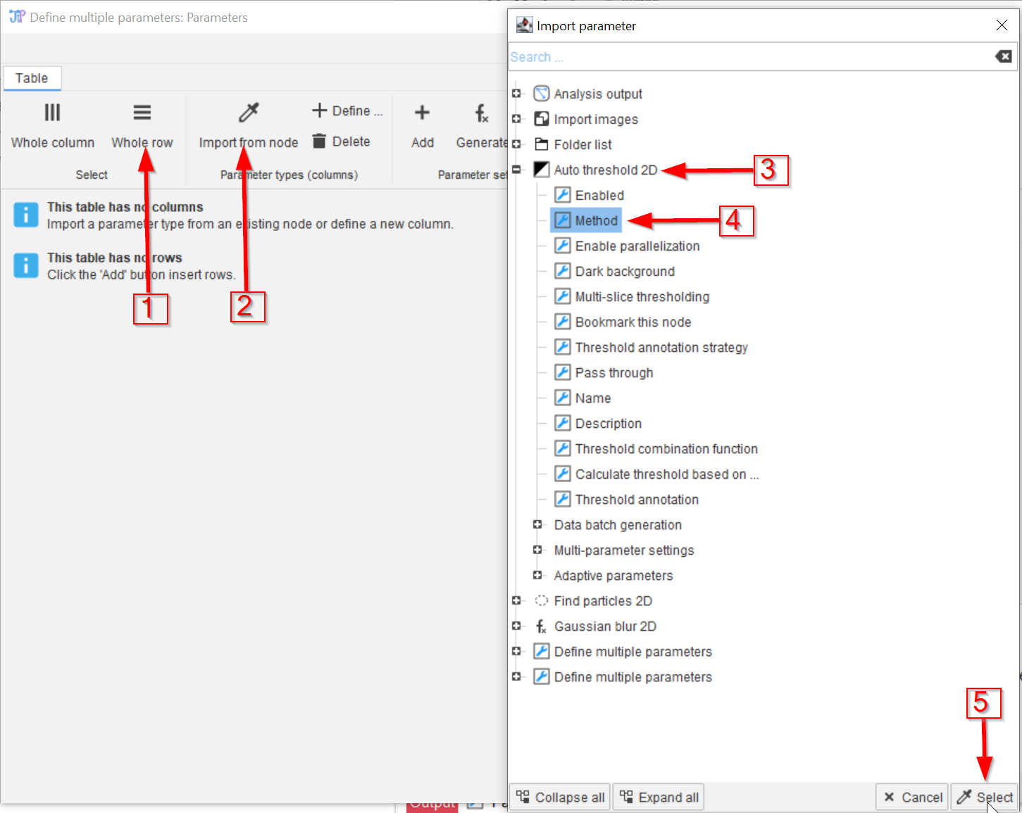
We begin by adding a new column by applying the following steps.
- To add a column ( = parameter) by selecting
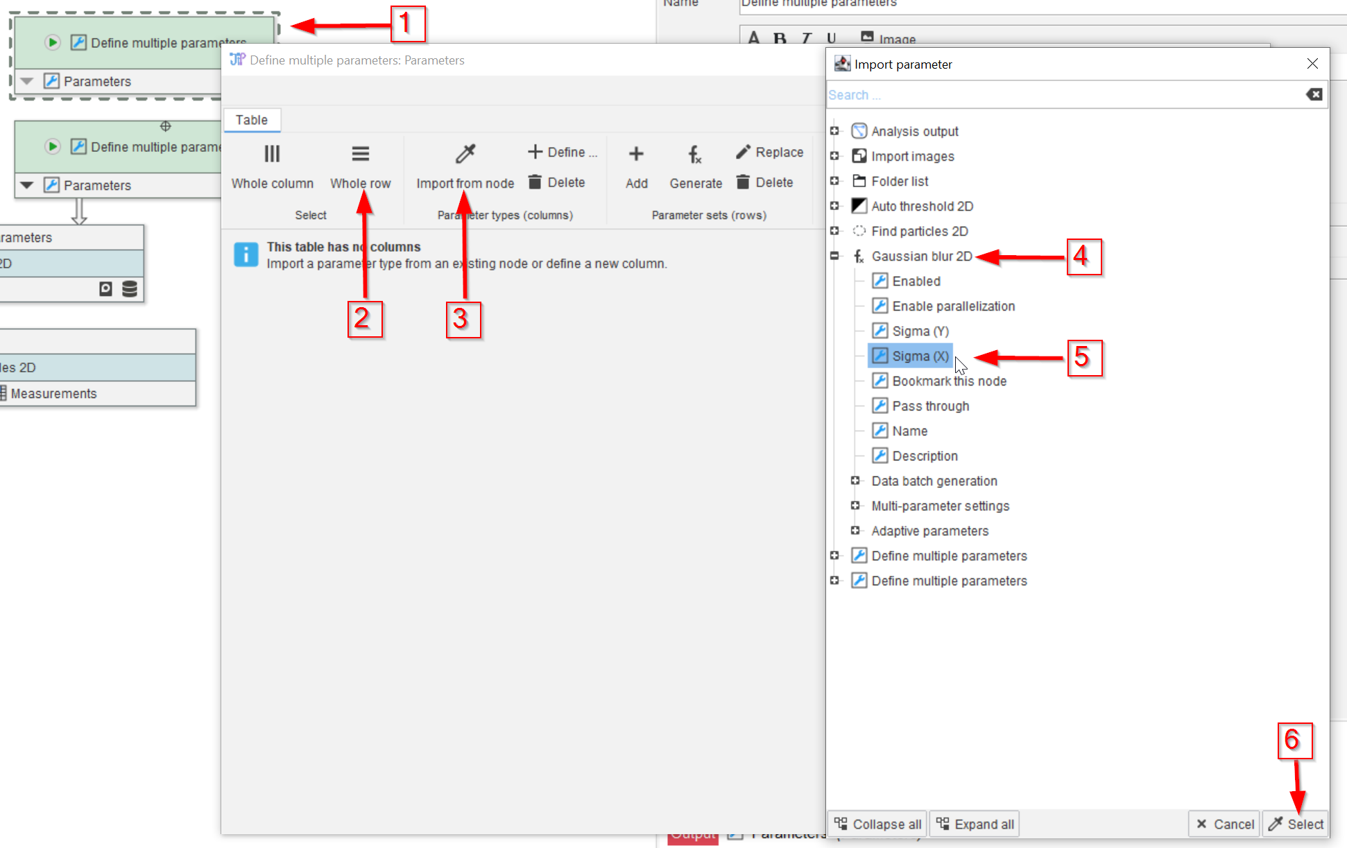
Import from node(red arrow 2), which will auto-configure a new column based on an existing node parameter - Find the
Auto threshold 2Dentry (red arrow 3) - Choose the
Methodparameter (red arrow 4) and select it (red arrow 5)

Step 5
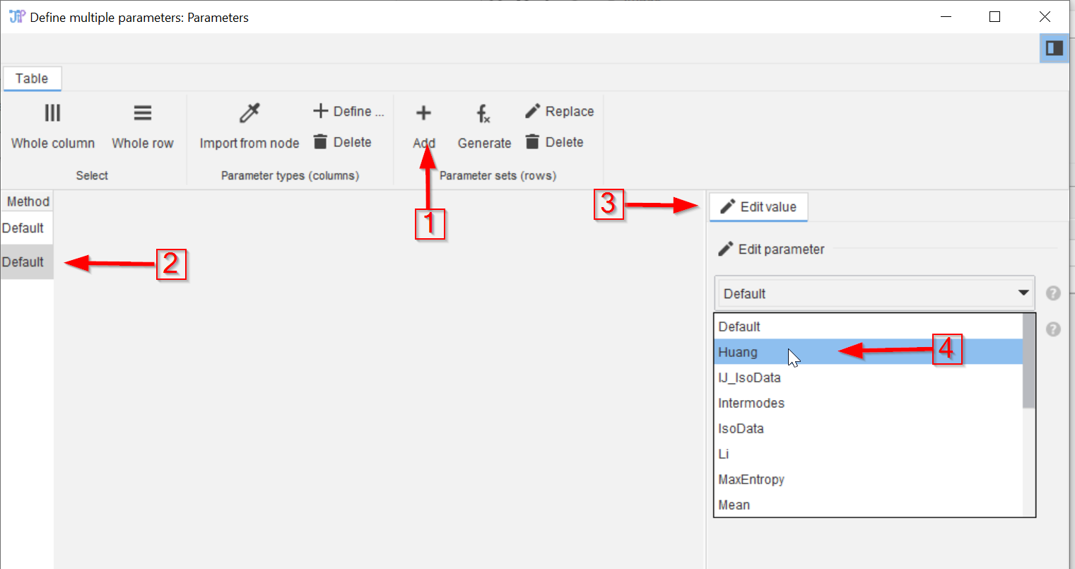
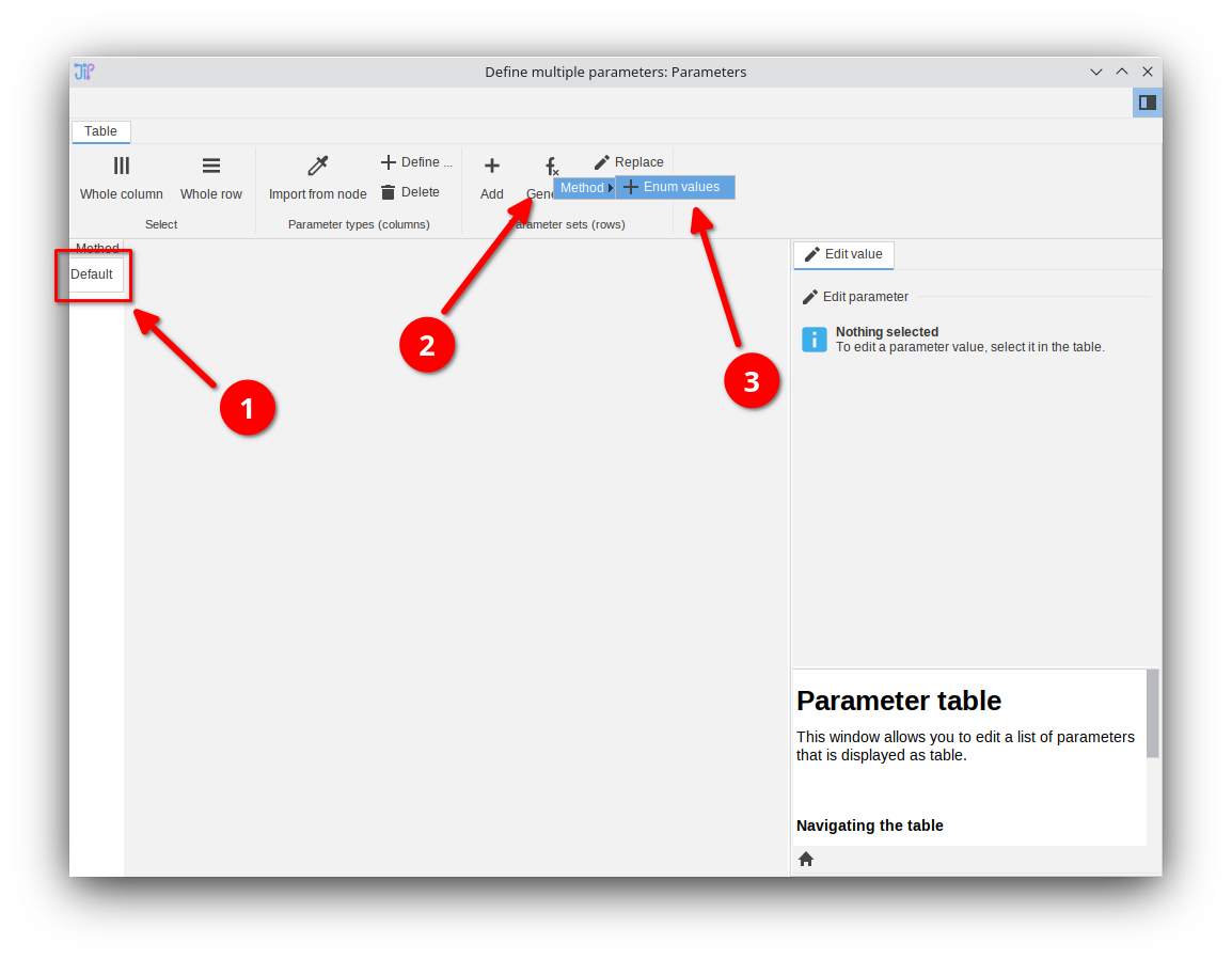
Click on Add (red arrow 1) to add a new row ( = parameter set), which will add the first thresholding method (Default) of ImageJ to the parameter list (red arrow 2).
Step 6
Repeat the process (red arrow 1) thus adding a second parameter set.
Select the 2nd entry (red arrow 2) and edit it (red arrow 3). Choose the next method (Huang) (red arrow 4) to change the entry to this value.
Step 7
If you want more entries, repeat the process until all the desired thresholding methods are n the parameters list (red rectangle 1).
Alternatively, you can let the editor generate all values automatically:
- Select one value of the column (note: there must be at least one parameter set)
- Navigate to
Generateand choose a generator (for theMethodparameter there is only one)
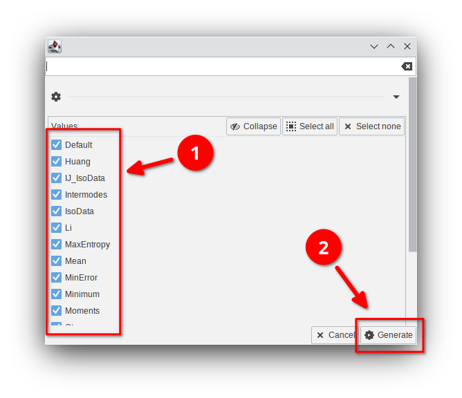
Step 8
Choose the parameter values that should be added as new parameter set.
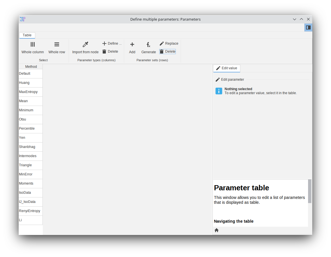
Step 9
Notice how now all thresholding options are setup.
Step 10
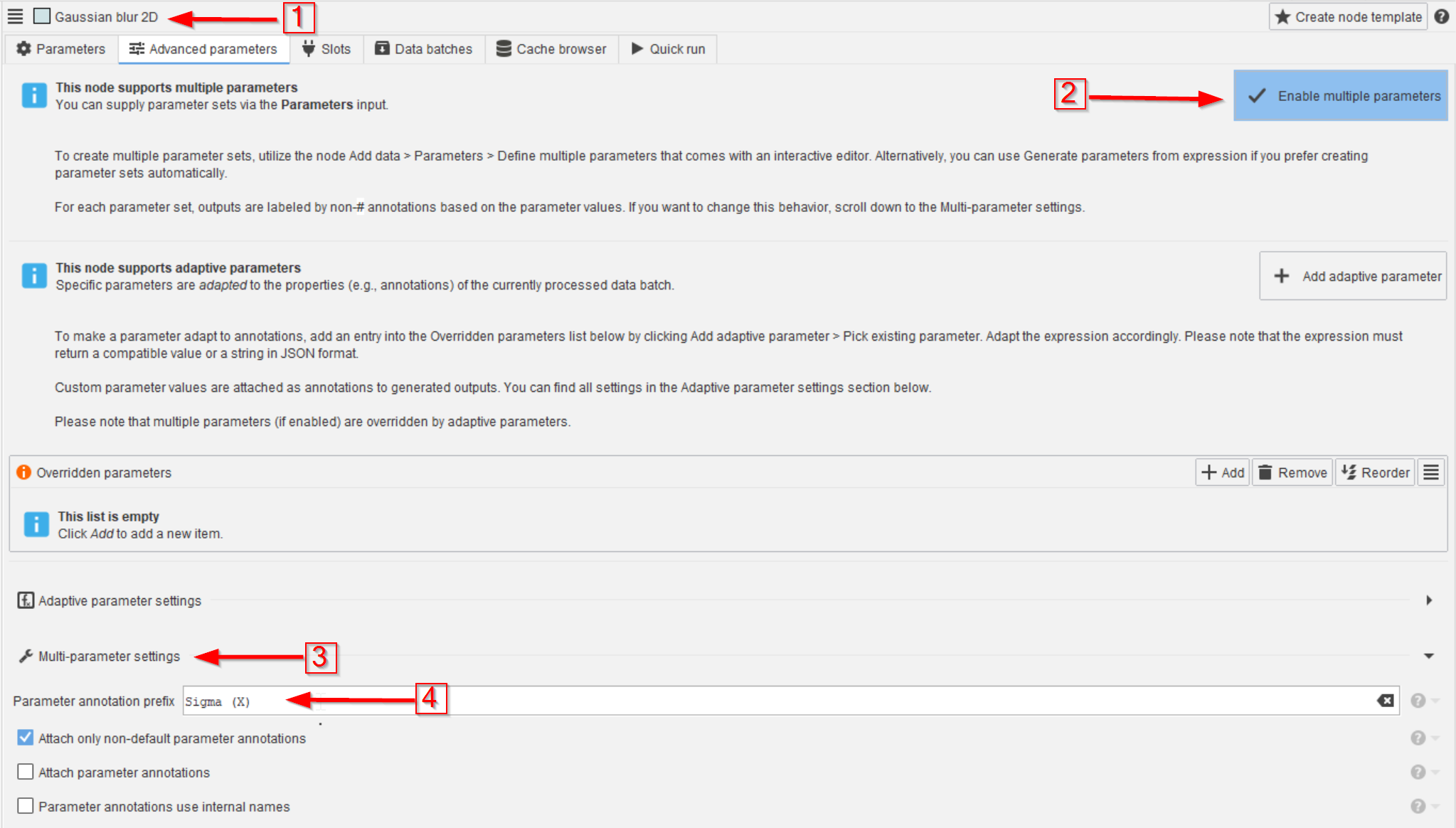
With the parameter sets now configured, select the Auto threshold 2D node.
Now select the Advanced parameters tab and enable the multiple parameters mode (red arrow 2).
By default, the multi-parameter mode will automatically attach all externally set parameters to the generated data. The name of the annotation is automatically generated, but can be prefixed with a custom string by the setting Parameter annotation prefix (red arrow 4).
You can leave the Parameter annotation prefix empty.
Step 11
This action opens a new input slot Parameters on the threshold node (red arrow 1), which can be connected to the Define multiple parameters node (red arrow 2).
Step 12
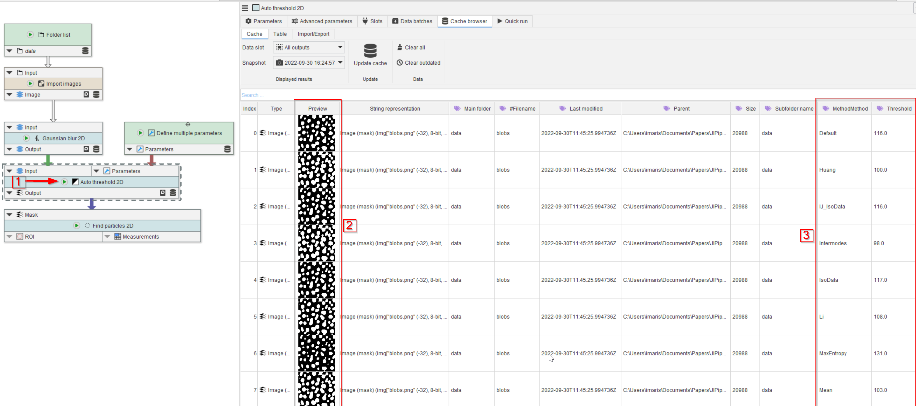
Run the threshold node (red arrow 1) and observe that the cache now contains as many images as the number of selected threshold methods (red rectangle 2).
The name of the method and the threshold value also appear as annotations (red rectangle 3).
Here it is named “MethodMethod”, because we set the prefix to “Method”
Step 13
Let’s proceed by generating multiple parameters for the Gaussian blur.
The addition of number-type multiple parameters works very similarly.
Add another node Define multiple parameters (red arrow 1) which will be used with the Gaussian Blur 2D, controlling the Sigma (X) parameter.
Add a whole row (red arrow 2), import from a node (red arrow 3), select the Gaussian Blur 2D entry (red arrow 4) and choose Sigma (X) (red arrow 5). Accept the choice (red arrow 6).
Step 14
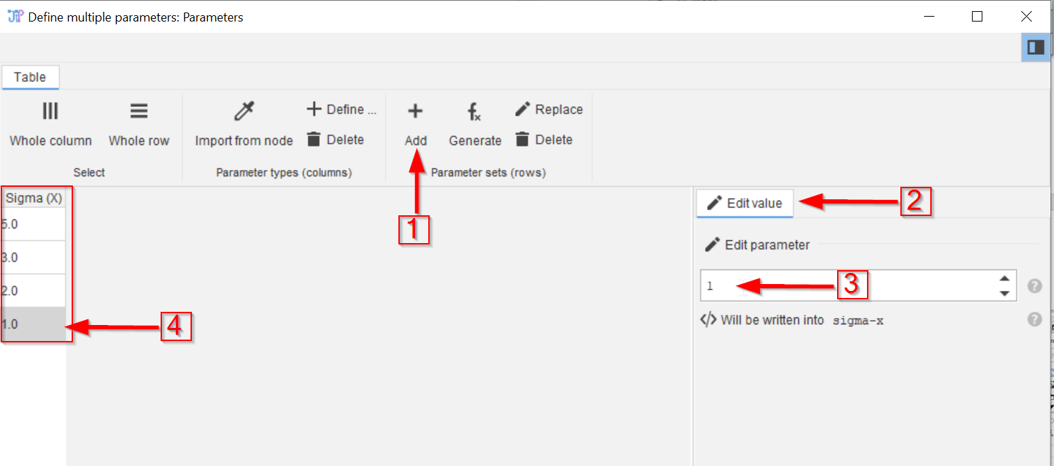
Add more values (red arrow 1), edit their values (red arrow 2) b y setting the desired sigmas (red arrow 3), which will appear in the list (red arrow 4, red rectangle).

Step 15
In the Gaussian blur 2D node (red arrow 1) enable multiple parameters (red arrow 2), and use the parameter setting (red arrow 3).
Here you can again provide a prefix if you want (red arrow 4).
Step 16
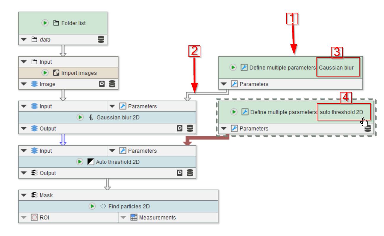
Connect the new parameter node (red arrow 1) to the Gaussian blur node (red arrow 2). Feel free to adjust the names of the parameter nodes to indicate their target (red rectangles 3 and 4).
Run the nodes and observe that now we have 32 results (a combination of 4 gaussian sigmas and 8 threshold methods). Study the outcome of the Find particles node in terms of how these parameters affect the number of identified ROIs.