Working with the cache: managing and exporting

Summary

Explains how to manage the cache and export cached data into the standard JIPipe format.

Tutorial data

This tutorial has accompanying data. Please download the data if you want to follow the guide.

Tutorial

Project + Data

Preliminary steps

Please ensure that you have look at the previous tutorial.

View previous tutorial

Step 1

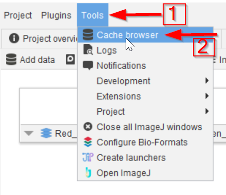
Load the example pipeline.

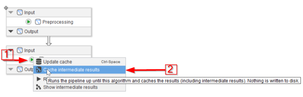
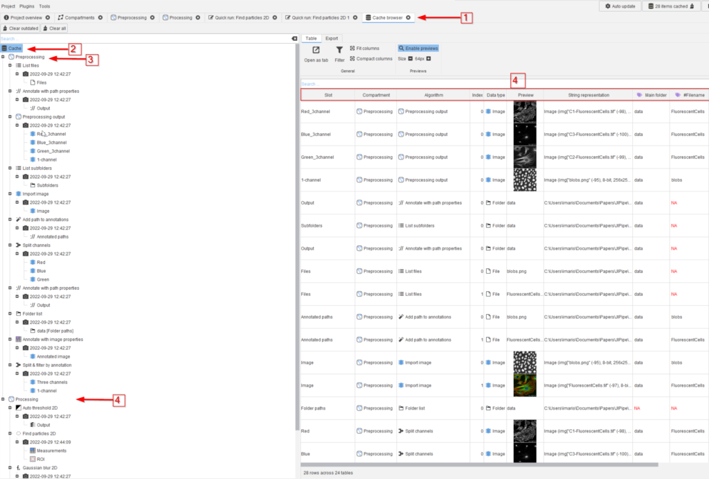
Go to the Compartments tab and update the cache directly from there. This can be achieved with the compartment nodes the same way as with regular nodes. Use the green arrow on the Processing compartment (red arrow 1) and choose the Cache intermediate results option to save the cache for all nodes (red arrow 2).

Step 2

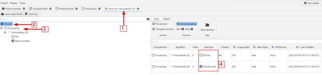
In the Cache browser tab (red arrow 1), the presented results can be filtered via the search field (red arrow 2).

Step 3

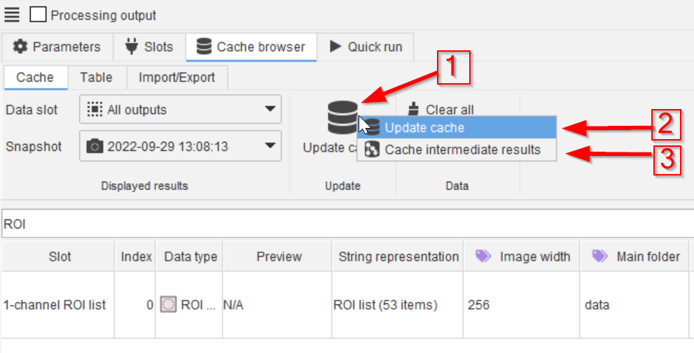
E.g., looking only for ROI data, we can use the search term ROI in the search field (red arrow 1), and see only the ROI results.

Step 4

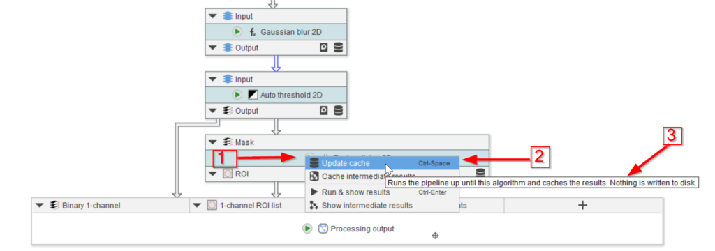
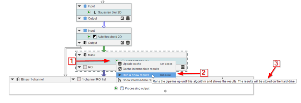
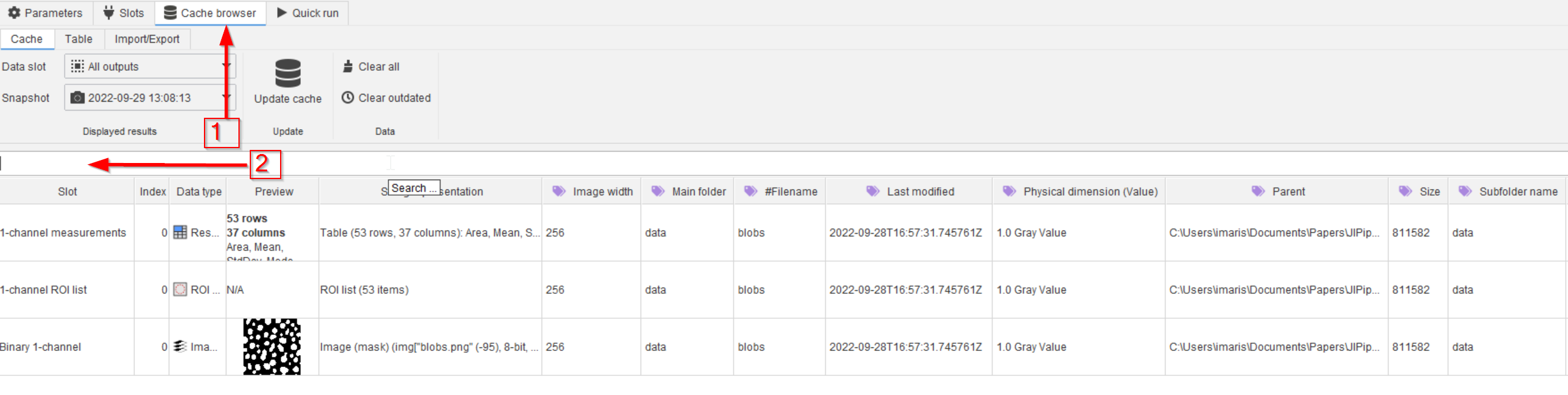
Updating the cache of the specified node is also possible directly from here (red arrow 1) using the usual two options (red arrow 2 and 3).

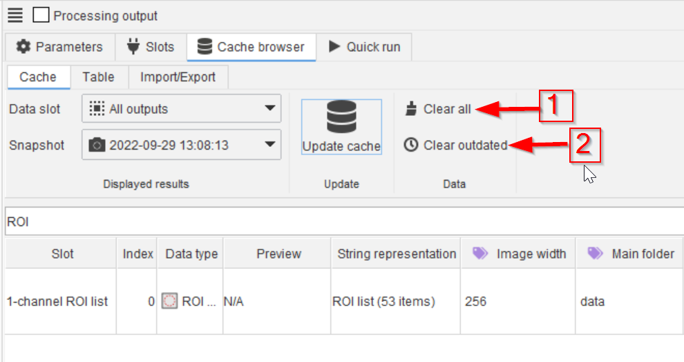
Step 5

Similarly to the project-wide cache browser tab, clearing the cache is also possible from this window, aiming either at all cache content (red arrow 2), or only at the outdated content (red arrow 3).

Info

Cached data is outdated if its producing nodes (or their predecessors) were deleted or have different parameters compared to when the data was generated.
For example, if a predecessor Gaussian blur 2D node’s sigma value is changed, all successor node’s cached data is marked as outdated.

Step 6

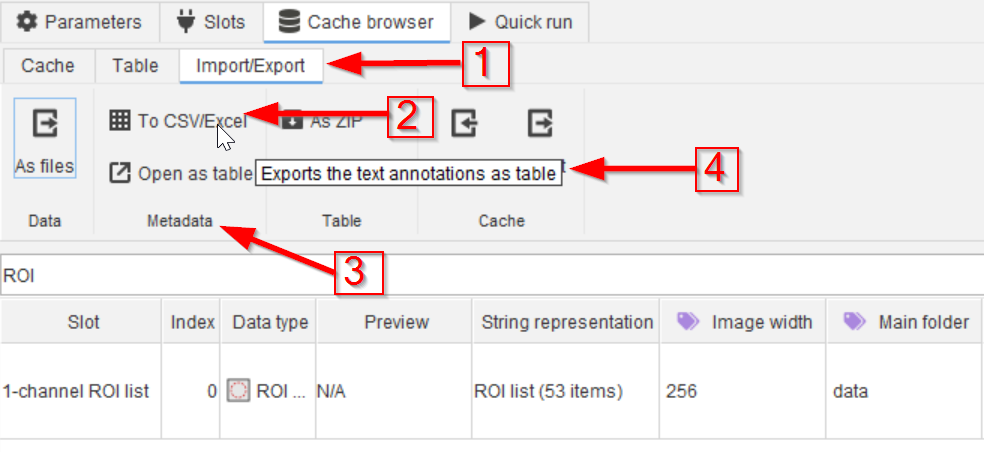
Exporting the cache and its metadata can also be carried out via simple options.

Use the Import/Export tab (red arrow 1), choose e.g., the CSV/Excel option (red arrow 2) which will refer to the metadata (red arrow 3) and it will export the text annotations as a table (red arrow 4).

Info

Exporting the metadata will yield a table with all information displayed in the cache browser table, excluding the underlying data (e.g., images, ROIs, …).

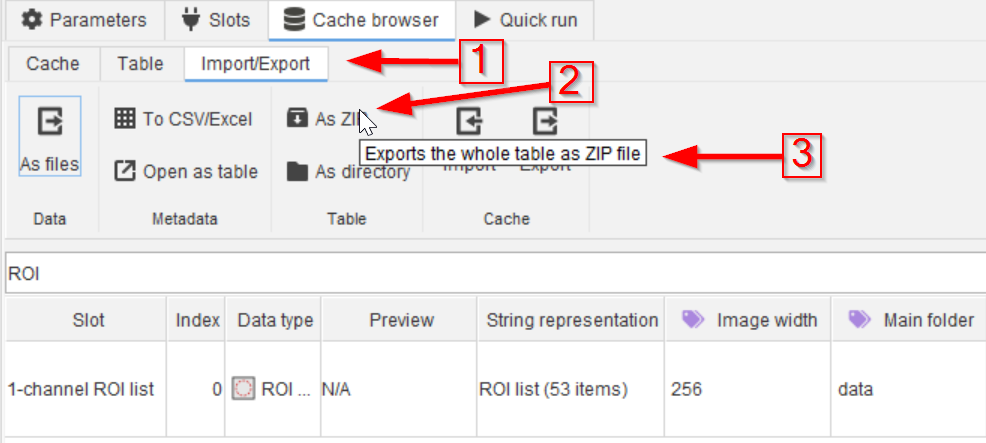
Step 7

Another Import/Export option (red arrow 1) is saving a ZIP file (red arrow 2) of the entire dataset (red arrow 3).

Info

The generated ZIP file (or directory if the other option is chosen) will contain the displayed table, including its metadata and data in a standardized JIPipe format.
While the format can be browsed by humans, it is mainly designed for reading via a program. The export of data into a format more suitable for humans will be handled in a later tutorial.

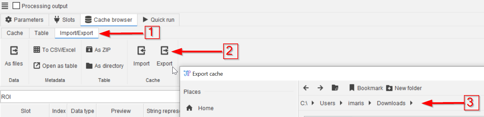
Step 8

The Import/Export menu (red arrow 1) also allows the importing/exporting of the entire cache of the selected node (red arrow 2) to a selected/created directory (red arrow 3).

Info

The difference between exporting the current table (as indicated by the Table label) and the whole node cache is that the full-cache options store all outputs of the node, while the Table-functions exclude all non-selected outputs.

Step 9

The exported cache contains a machine-readable and heavily structured design of all results, which can be navigated to automatically by following the pop-up link (red arrow 1).

Step 10

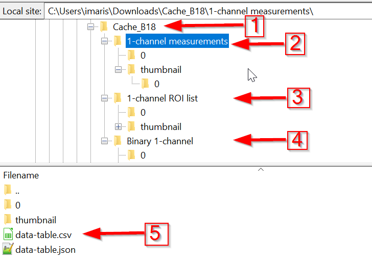
Under the folder name (red arrow 1), the groups of results are listed (red arrow 2-4), as they appeared in the cache. Inside each of the entries, data-table.csv and data-table.json files (red arrow 5) explains the content of the data subfolders, and contains the metadata.

Info

Only the data-table.json file is relevant for importing metadata. The data-table.csv table is generated for the sake of convenience.

Step 11

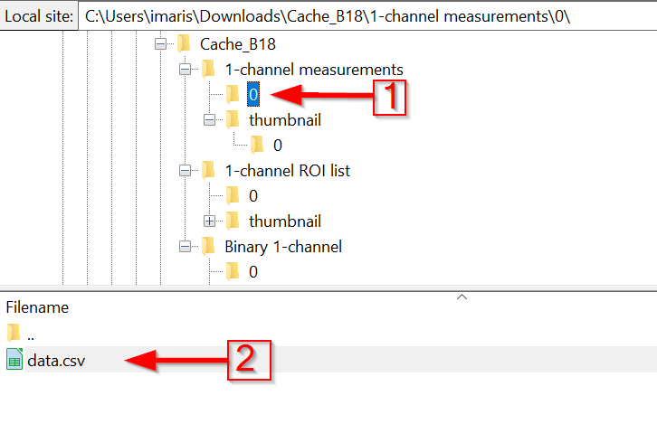
The numbered subfolder will contain the actual cached data of the 1-channel measurements output (red arrow 1) in a *.csv file (red arrow 2).

Info

The numeric folders are standardized. In JIPipe, navigate to Help > Data type compendium to review the exact specifications of the directory contents.

Step 12

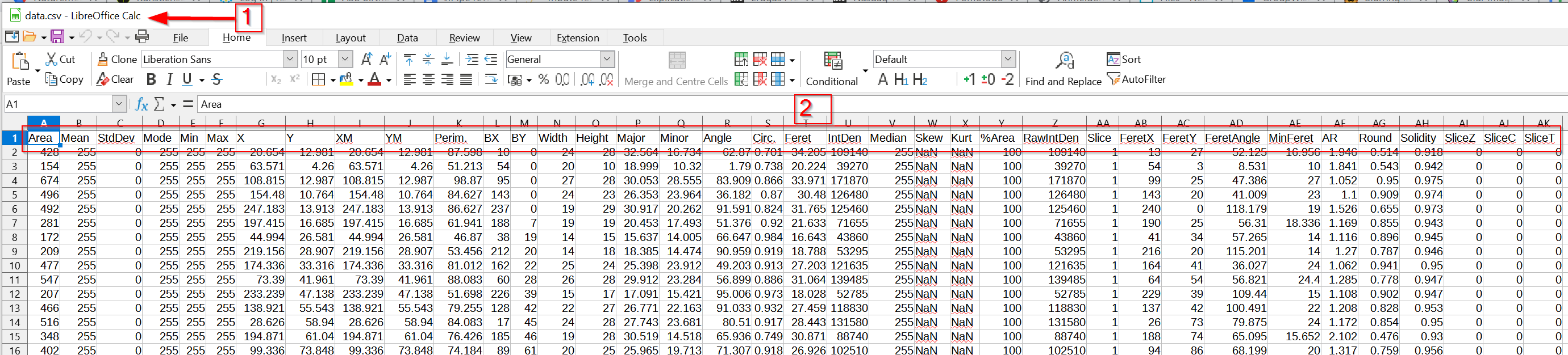
This file contains the cached results (red arrow 1), as observed in a spreadsheet viewer.

The results are organized in a columnar matter (red rectangle 2).