Step 1
Load the example pipeline.
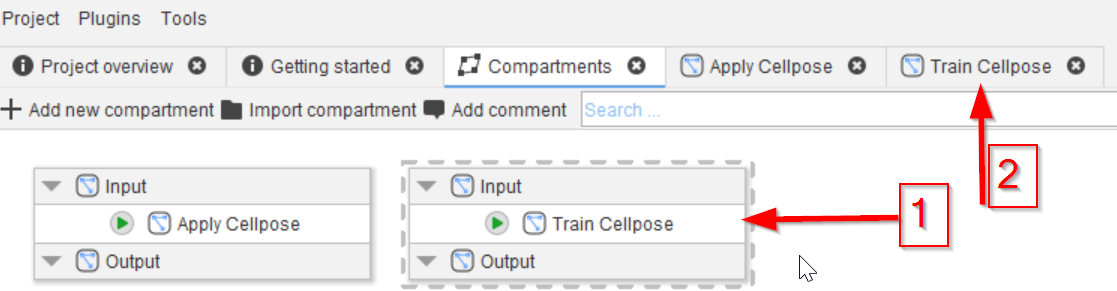
Add a second compartment, name it Train Cellpose (red arrow 1) and open it in a tab by double-clicking it (red arrow 2).
Step 2
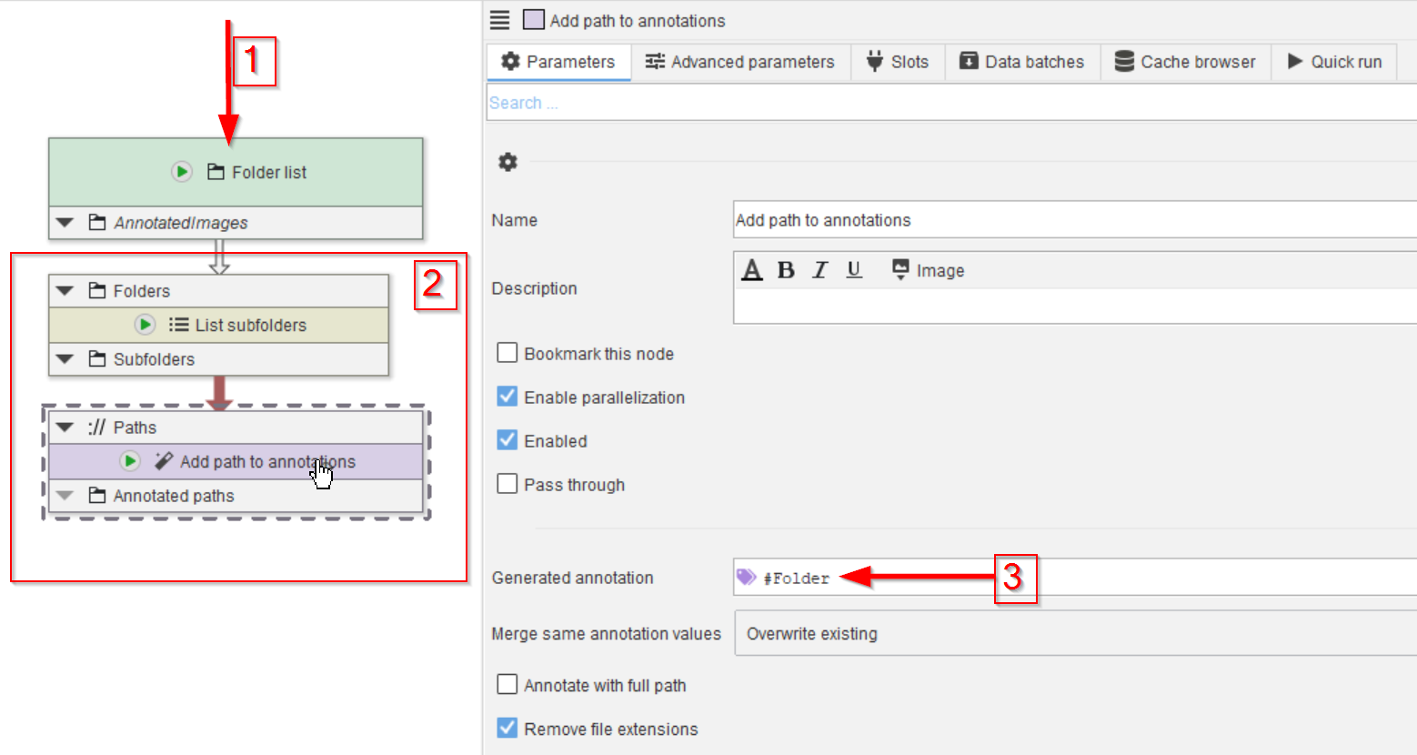
Drop the data folder on the UI (red arrow 1) and add the nodes List subfolders and Add path to annotations (red rectangle 2).
Configure the Add path to annotations to generate an annotation #Folder (red arrow 3). Note the # to make it recognizable by the data management system as mode to group data.

Step 3
Note that the training dataset (red arrow 1) consists of subfolders (red arrow 2) with matching pairs of TIFF and ZIP files (note 3).
The latter contains the manually annotated objects as ROIs, designed to be used by the Cellpose trainer.
Step 4
Accordingly, we need to read the TIFF and ZIP files separately.
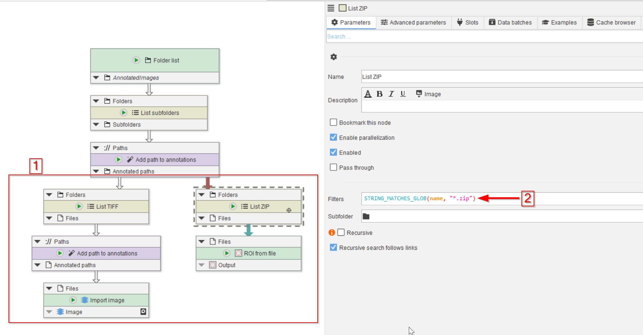
This can be achieved by establishing two branches, one each for the two file types by the introduction of two List files nodes that we renamed to List TIFF and List ZIP in our figure (red rectangle 1).
The List files node can be configured with a filter expression to only detect specific files. In the case of the the List ZIP node, set the expression to
STRING_MATCHES_GLOB(name, "*.zip")For List TIFF, set the expression to
STRING_MATCHES_GLOB(name, "*.tif")After the List TIFF node, add another Add path to annotations to also save the image file name.
Step 5
Cellpose training requires label images or masks.
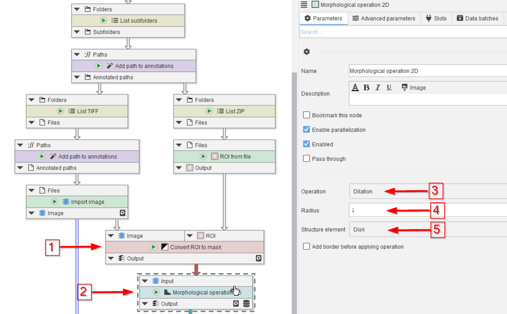
The can be created directly from ROI, for example via the node Convert ROI to mask, given the input image as reference (red arrow 1).
The generated mask will be dilated before being used for the Cellpose training (red arrow 2). The dilation serves the purpose of adding environment to the manual annotations, which should help the learning process (red arrows 3-5).
Setting the Radius parameter (red arrow 4) to various values may help to optimize the learning process.
Step 6
We continue with assigning the annotation masks to the actual images.
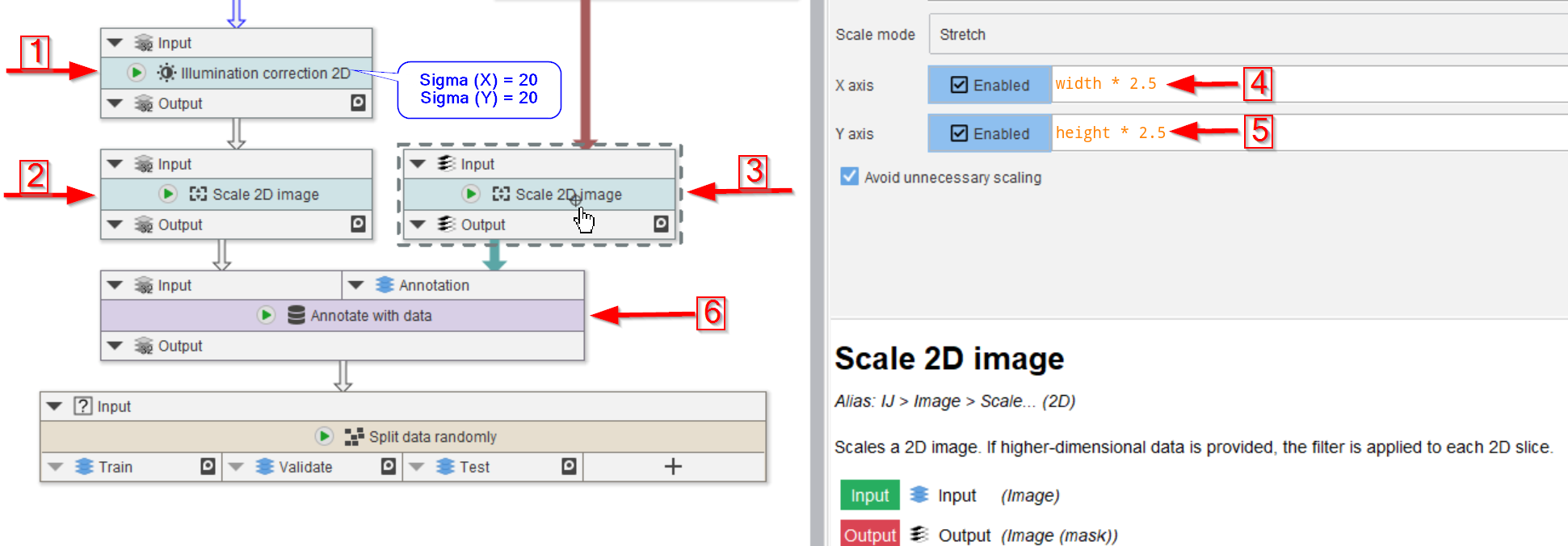
In preparation for this, we first correct the image for illumination inhomogeneities via Illumination correction 2D (red arrow 1), where we use 20 px radius for both Sigma (X) and Sigma (Y) in underlying Gaussian filter.
Both the image and the annotations are scaled (red arrows 2 and 3) with a factor of 2.5 (red arrow 4 and 5):
X axisset towidth * 2.5Y axisset toheight * 2.5
The raw image and the labels are now merged together via a data annotations.
Annotate with data is utilized to annotate each raw image with its corresponding mask (red arrow 6). This will generate a new column next to the text annotations that can be read by the Cellpose training node.
Finally, connect the annotated data to a node Split data randomly (percentage).
Step 7
Use the slot editing capabilities of Split data randomly (percentage) to create the following output slots of type Image:
TrainValidateTest
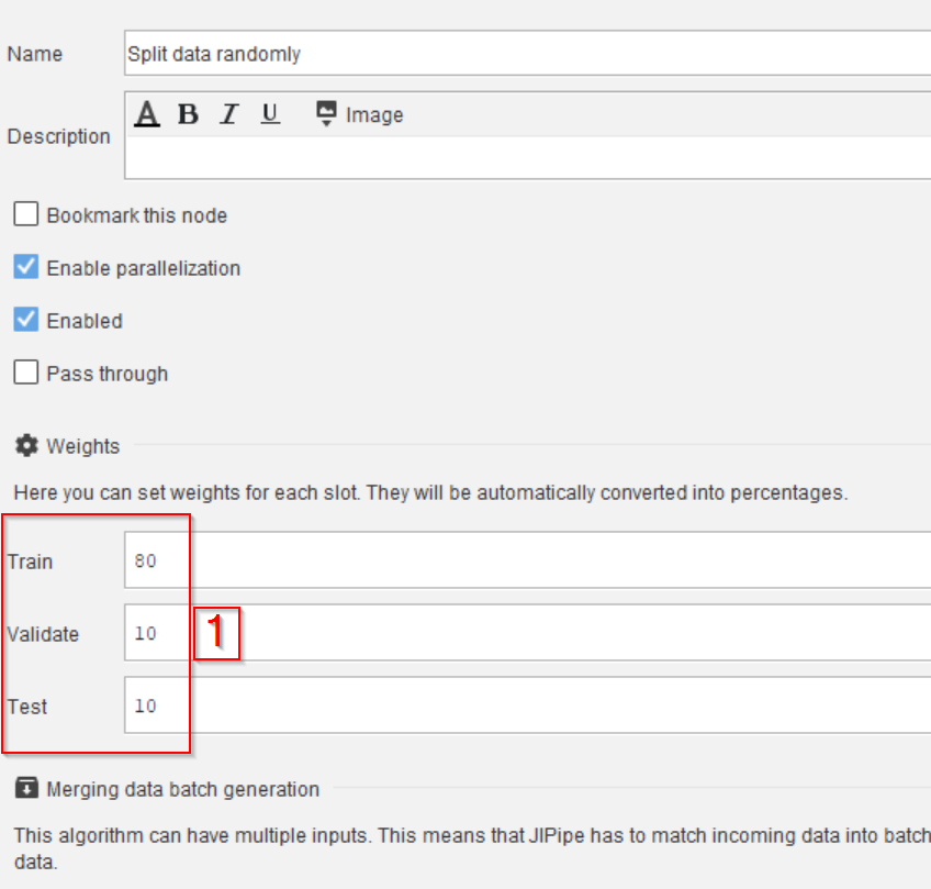
Then configure the percentages in the Parameters tab and the Weights category (red rectangle 1) as following:
Trainset to80Validateset to10Testset to10
Step 8
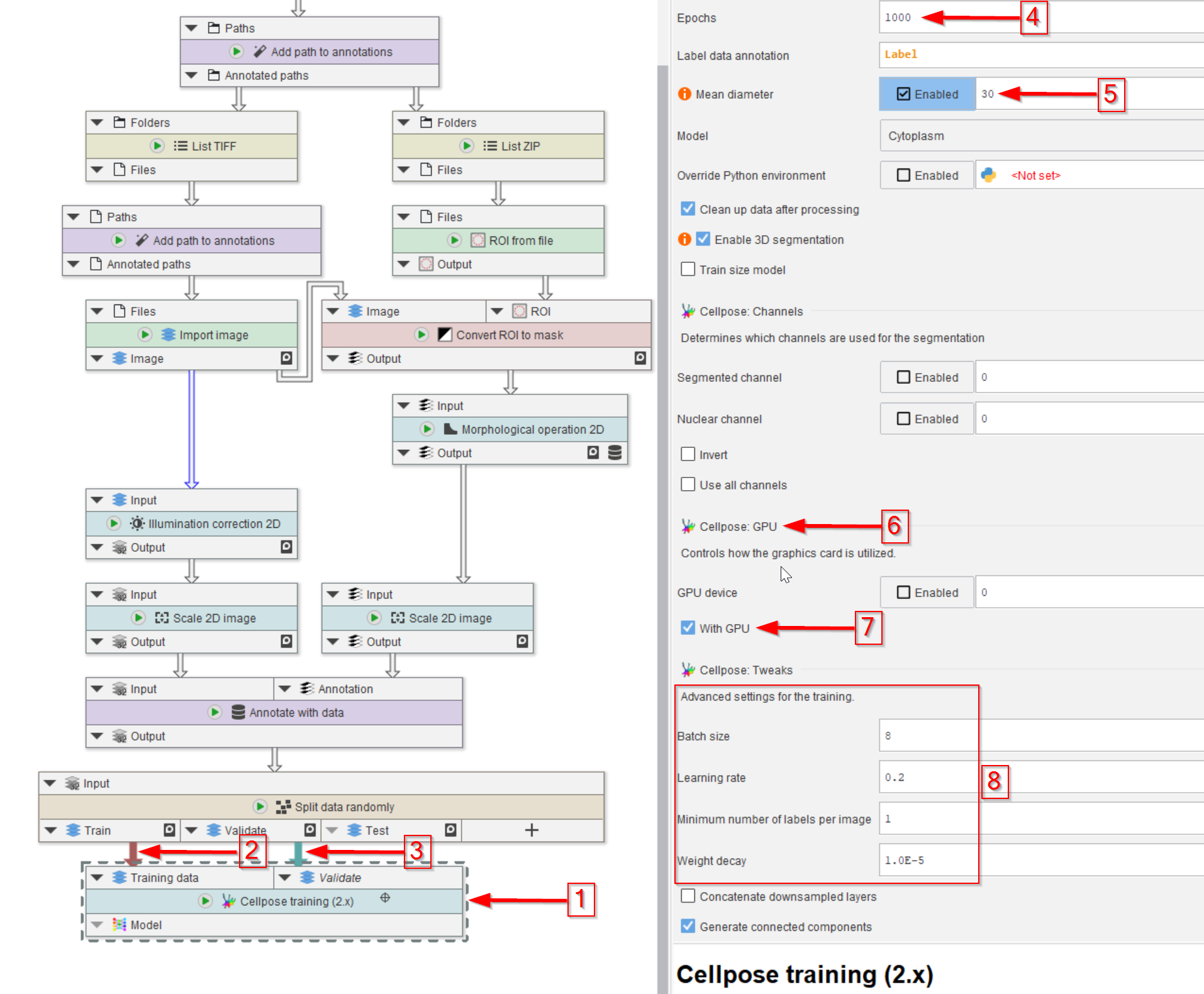
The Cellpose training (2.x) node is then added (red arrow 1) and connected to the training (red arrow 2) and validation (red arrow 3) output of the Split data randomly (percentage) node.
The number of training epochs (red arrow 4) and the mean diameter of the object that we seek (red arrow 5) are the most important setting here.
Make sure to activate the GPU if the PC has one (red arrow 6 and 7) to expedite the learning process.
Finally, the training setting can be easily adjusted in the UI (red rectangle 8).

Step 9
The trained model can be saved from the cache browser (see Tutorial), and it can be used directly to visualize the segmentation quality using the test dataset.
For the latter, use the output model of the training node (red arrow 1) to guide a Cellpose (2.x) node (red arrow 2) via connecting the newly trained model to the corresponding input of the Cellpose (2.x) node (red arrow 3).
The data input of the Cellpose (2.x) node (red arrow 4) will come from the test output of the random data splitter (red arrow 5).
In the Cellpose (2.x) node parameters, set the diameter to the same value as the model (red rectangle 6).
Very importantly, set the Model to Custom (red arrow 7, red rectangle) to have the Cellpose node accept an outside model connection.

Step 10
In order to utilize a saved model drag the Cellpose model file (a file with a very long name) into JIPipe. This will create a File list node as usual.
Alternatively, you can also create a File list node manually and use the file browser to select the Cellpose mode (red arrows).
Step 11
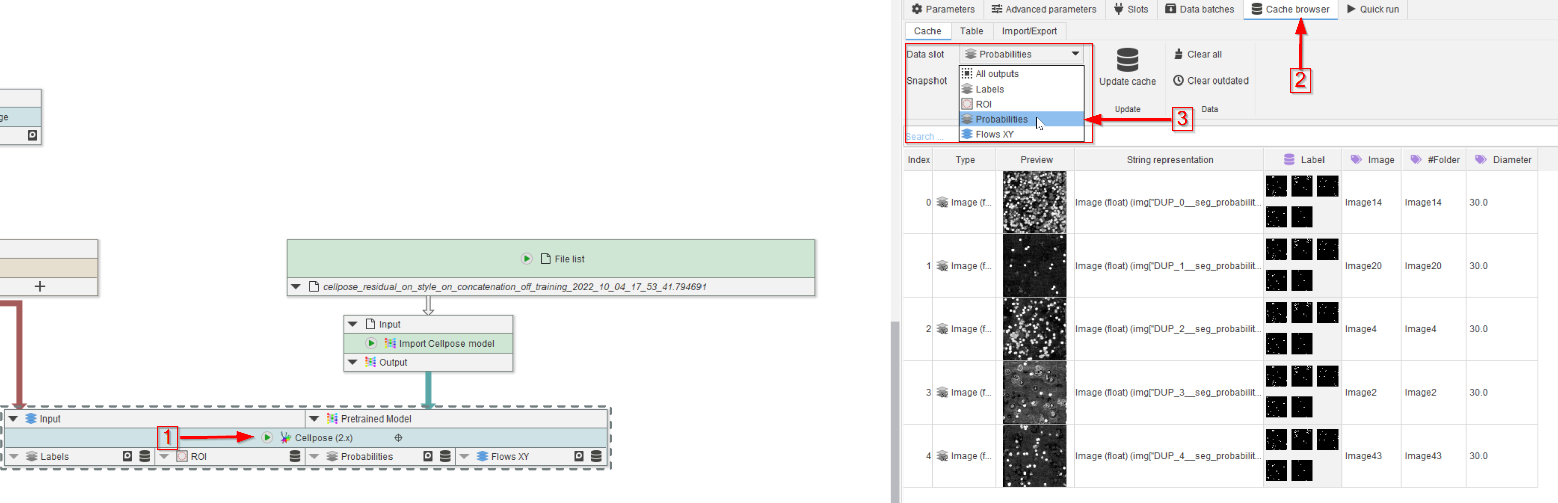
Run the node (red arrow 1) and observe the Cache browser (red arrow 2). The segmented peroxisomes are now illustrated by the selected outputs of the Cellpose (2.x) node, e.g., in this example, we set Labels, ROI, Probabilities and XY flows as outputs (red rectangle), and selected Probabilities to be displayed (red arrow 3).
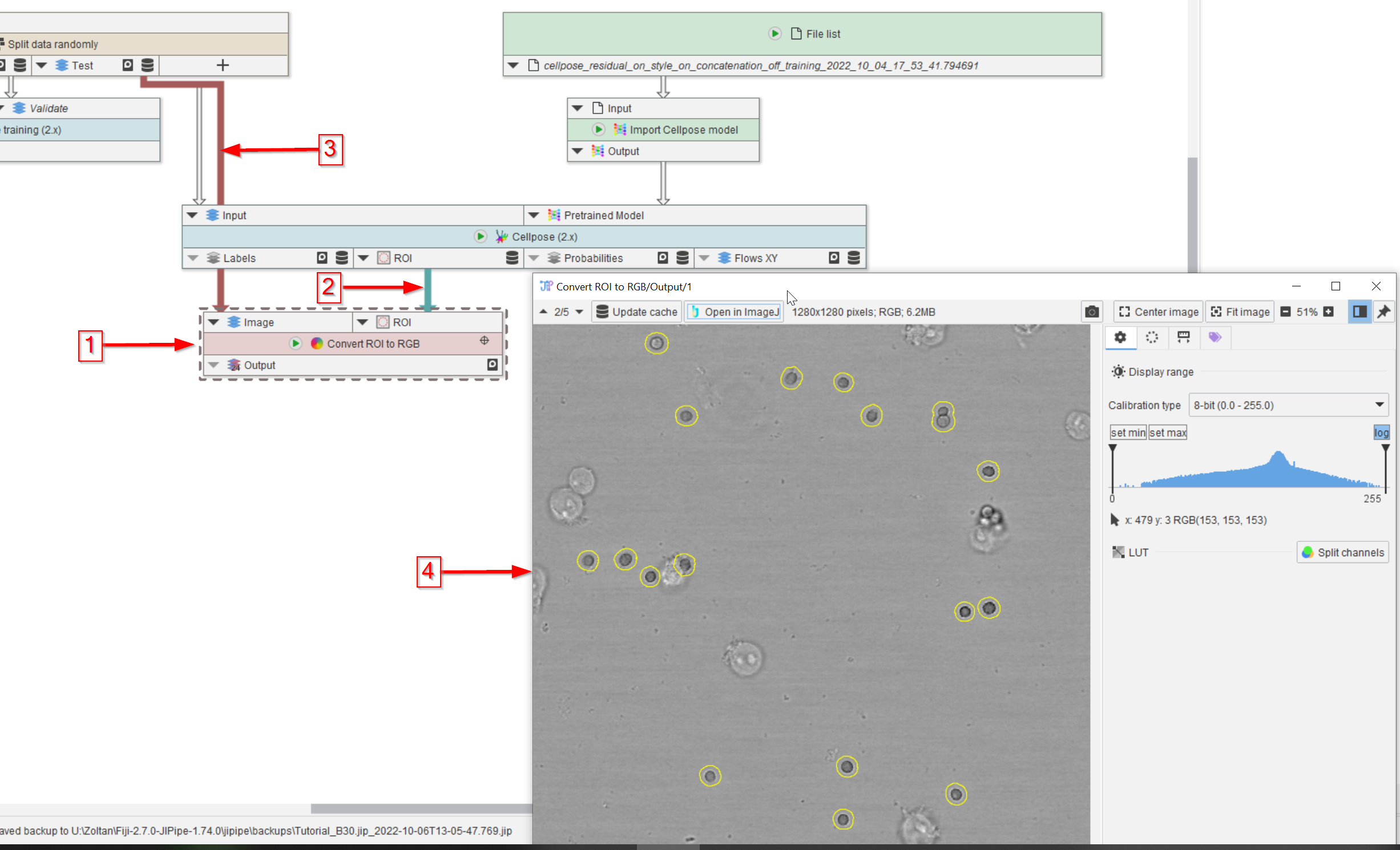
Step 12
To check the quality of the segmentation results visually, add a Convert ROI to RGB node to the UI (red arrow 1), connect it to the ROI output of the Cellpose (2.x) node (red arrow 2) and to the Test dataset (red arrow 3) of the Split data randomly (Percentage) node.
Observe the output in a viewer (red arrow 4) and notice the high quality of the segmentation (yellow circles outlining the peroxisomes).