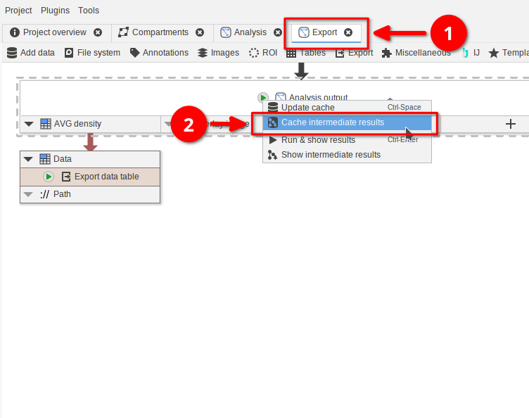
Step 1
Open the example project and navigate to the Export compartment (red arrow 1).
Update the cache using the output node’s Cache intermediate results option (red arrow 2).
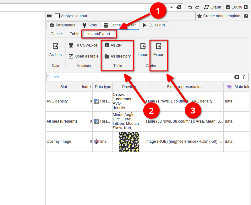
Step 2
In the Cache browser switch to the Import/Export tab (red arrow 1). Here you can manually export data into a JIPipe-compatible format. You have two options:
- Exporting the the currently viewed table of data (red arrow 2) as ZIP or directory
- Exporting the cache of the whole node (red arrow 3) as directory
The difference between these options is that the cache export ensures that you can later load in the result back into the current node via the Import function in the Cache section. To enable this, JIPipe saves multiple tables and additional metadata.
👉 Try to export the table as ZIP and directory, as well as exporting the cache.

Step 3
JIPipe comes with a node that allows the automated export of data into the standardized format.
This can be achieved by adding (red arrow 1) the node Export data table and connecting it to the output of any node (red arrow 2).
For example, we connected the node to the AVG density output of the Analysis output.
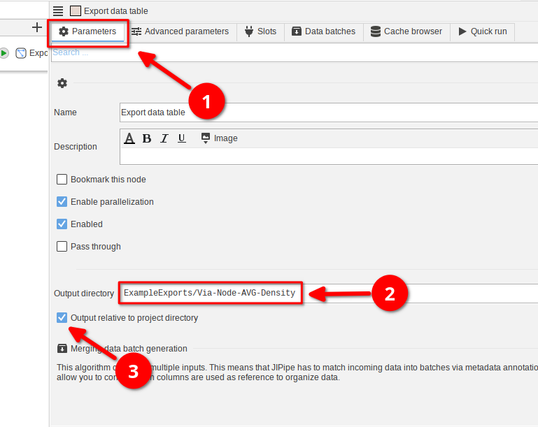
Step 4
By default, the Export data table node will store its output inside a automatically generated directory relative to the current output path (for cache runs it is in a temporary directory.
Alternatively, you can provide a custom path or one that is relative to the project directory:
To do this, select the Export data table node and navigate to the Parameters tab (red arrow 1).
Provide a relative output directory (i.e. does not start with / on macOS/Linux or with a drive letter on Windows; red arrow 2). Then enable the setting Output relative to project directory (red arrow 3).
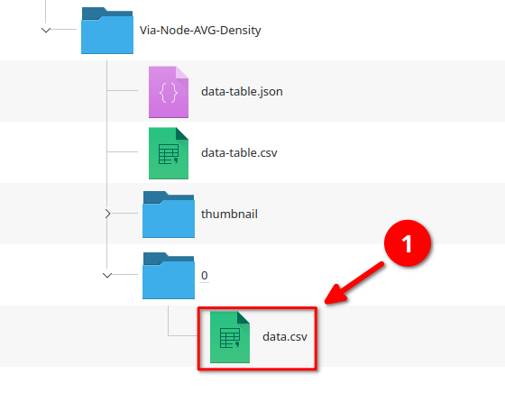
Step 5
Running the Export data table node now generates a directory next to the project file that follows the standardized JIPipe output format.
The actual data is contained in the data.csv file in the 0 directory (because it is the first row of the data table; red arrow 1). All other files contain the metadata.
Step 6
A benefit of the machine-readable JIPipe format is that all contained data and metadata can be conveniently restored by JIPipe.
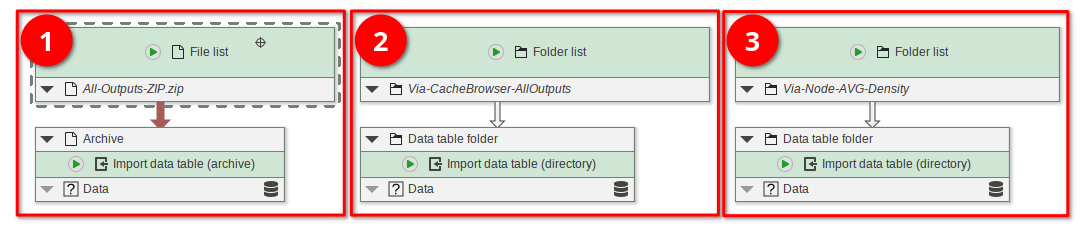
Open the Tutorial_B22-1_Part1.jip project that comes pre-loaded with nodes that cover various import scenarios:
The node Import data table (archive) (red rectangle 1) can import a ZIP file generated by the cache browsers’ ZIP-exporter function.
If the data is stored inside a directory (or if you just extract the ZIP), use the Import data table (directory) node (red rectangle 2 and 3). In the example pipeline, we import both the All outputs export generated by the cache browser, and the AVG-Density output that was exported via the node.
Step 2
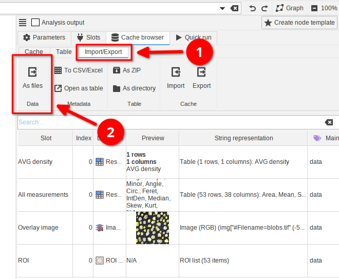
In the Cache browser switch to the Import/Export tab (red arrow 1). Here you can manually export data into a list of files based on the existing annotations.
Click the As files button in the Data category.
Step 3
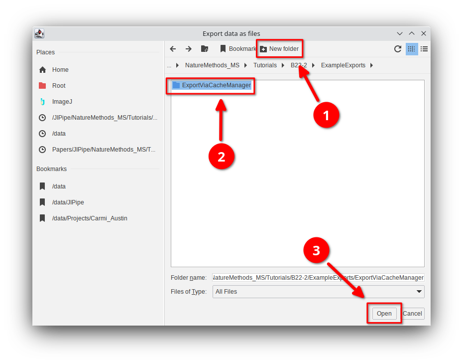
We recommend to create an empty directory for the storage of the exported data (red arrows 1 and 2).
Then choose the directory and click Open.
Step 4
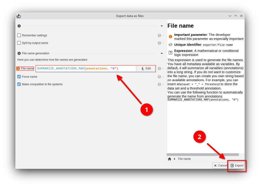
Now JIPipe will give you options that determine how the file names should be generated. This is required, as JIPipe does not know anymore the name of the original input file unless it is stored in the annotations.
The most important setting is the File name expression that defaults to
SUMMARIZE_ANNOTATIONS_MAP(annotations, "#")The expression is applied for each exported data item and returns the file name that should be used. The default method will take all known annotations that are marked with a # and form a filename based on the following pattern:
[Annotation 1 name]=[Annotation 1 value]If you want to know more about SUMMARIZE_ANNOTATIONS_MAP, please click Edit and search for the function in the function list.
In this case, you can leave the setting as-is.
Step 5
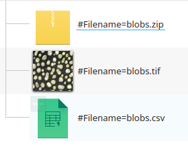
Open the directory after the export. You see that the exporter stored the data into an appropriate format.
You can also clearly see the pattern [Annotation 1 name]=[Annotation 1 value] as determined by the expression.
Step 6
JIPipe offers various nodes for the export of data that are even outside the scope of the exporter implemented in the cache browser.
You can find them in the Export menu or via the search bar.
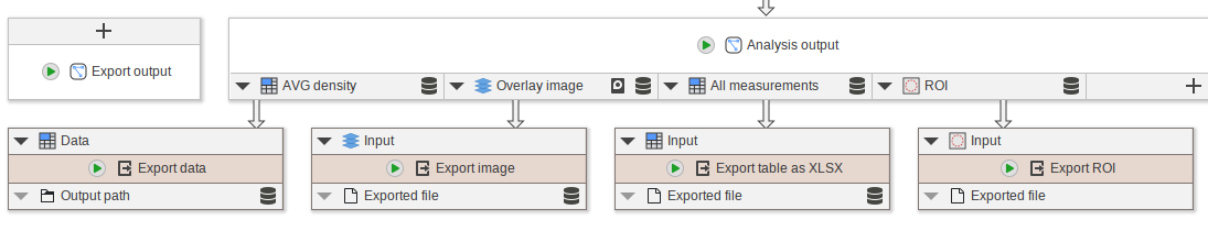
Proceed to add and connect the following nodes:
- Add
Export dataand connect it toAVG density - Add
Export imageand connect it toOverlay image - Add
Export table as XLSXand connect it toAll measurements - Add
Export ROIand connect it toROI
In the following steps, we will show how to configure these nodes for the export into a single directory.
Step 7
We begin with the Export data node. It encapsulates the same functionality as the cache browser’s data exporter.
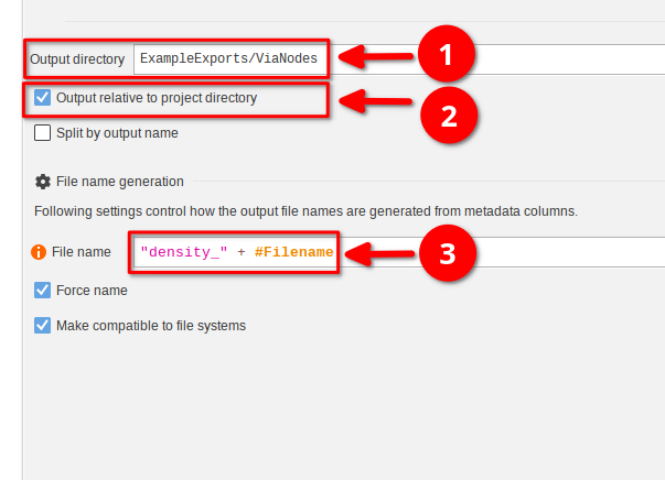
Here we will export the AVG density table into a directory ExampleExports/ViaNodes relative to the project file. Begin by selecting the node and changing the following parameters:
Output directorytoExampleExports/ViaNodes(red arrow 1)- Enable
Output relative to project directory. If this is not done, the files will be stored in a temporary directory (red arrow 2)
It is common that the type of the output is stored within the filename. To to this in JIPipe, modify the File name property as follows:
"density_" + #FilenameThe exporter will use the expression to determine the filename of each exported data item. As the images are annotated with a #Filename annotation, we can combine it with a custom text "density_" to generate files with that pattern.
Step 8
Run the Export data node via Update cache.
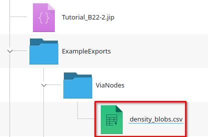
Now navigate to the ExampleExports/ViaNodes directory that should have appeared next to the project file. It contains a file density_blobs.csv according to the pattern defined by the File name expression:
"density_" plus #Filename, where #Filename is blobs, because the table was annotated with the original filename (blobs)
Step 9
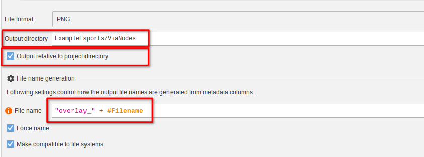
Select the Export image node and navigate to its parameters. Unlike the generic data exporter Export data, it allows you to change the output type of the generated file from TIFF to PNG or other formats.
Again, set the Output directory to ExampleExports/ViaNodes with Output relative to project directory enabled.
The filename expression set to
"overlay_" + #FilenameThis would yield a file that is for example named overlay_blobs.png.
Step 10
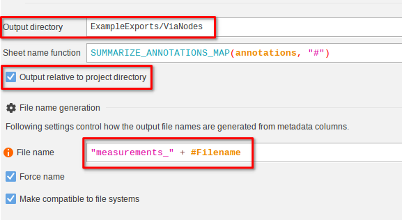
Move on to the Export table as XLSX node. While Export data will always export CSV files, this node will instead Excel files. It can even be configured to export multiple tables into one XLSX file.
Again, set the Output directory to ExampleExports/ViaNodes with Output relative to project directory enabled.
The filename expression set to
"measurements_" + #FilenameThis would yield a file that is for example named measurements_blobs.xlsx.

Step 11
Finally, edit the parameters of Export ROI node. Export data will export a *.roi file if only one ROI is present and otherwise compress all ROIs into a *.zip file. This node can optionally turn off this export behavior and export all ROIs into an individual *.roi file.
Again, set the Output directory to ExampleExports/ViaNodes with Output relative to project directory enabled.
The filename expression set to
"rois_" + #FilenameThis would yield a file that is for example named rois_blobs.zip or rois_blobs.roi depending on whether one or multiple ROIs are present.
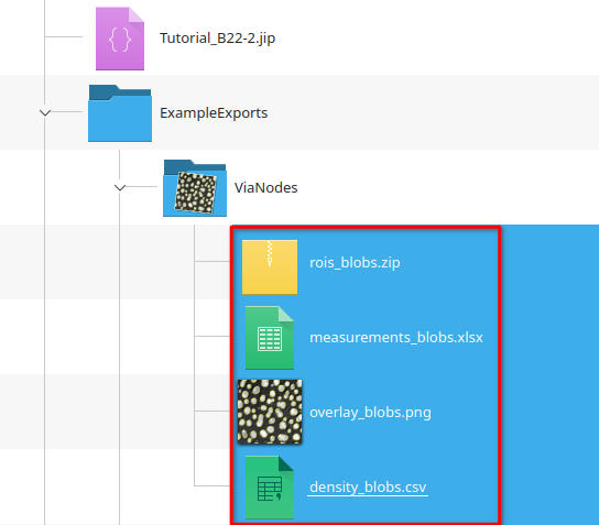
Step 12
Run all the exporter nodes via Update cache and navigate into the ExampleExports/ViaNodes/ directory.
Observe the generated files.