Processing ROI – JIPipe for ImageJ

Summary

Explains how to add new nodes via the algorithm finder into a project and use them to import an image file.

Tutorial data

This tutorial has accompanying data. Please download the data if you want to follow the guide.

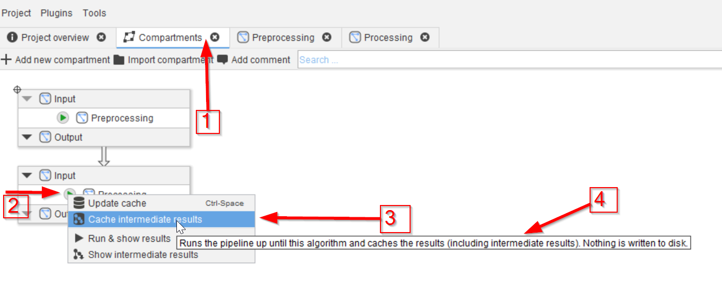
Step 1

Open the example pipeline, go to the Compartments tab (red arrow 1) and run the Process compartment (red arrow 2). Use the Cache intermediate results method (red arrow 3) to be able to see the cache content of all nodes in both compartments (red arrow 4).

Step 2

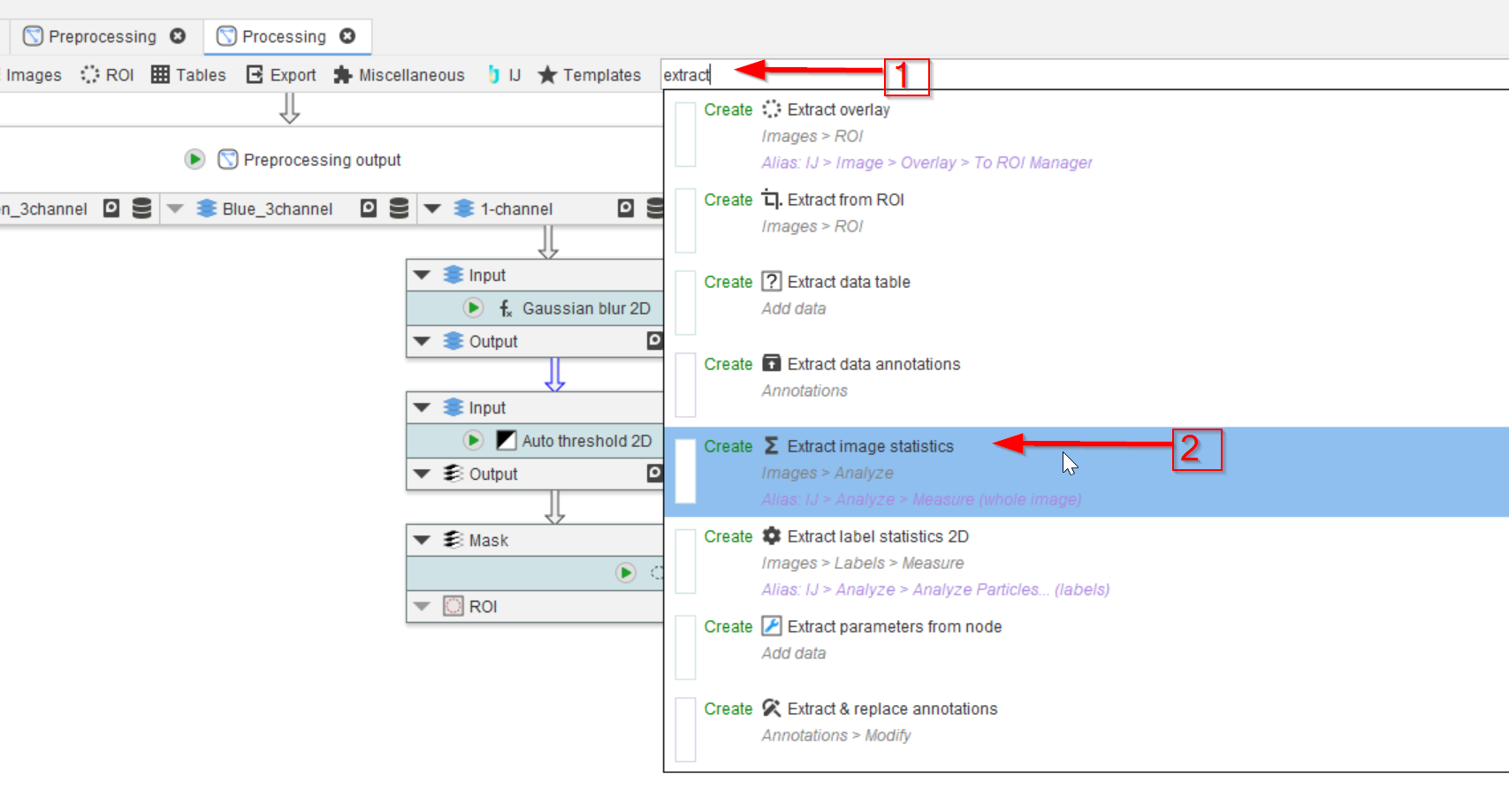
Step 3

Look for nodes with the name extract (red arrow 1) and choose the Extract image statistics node (red arrow 2).

Info

Extract image statistics measures statistics on the whole image or an optional ROI. It is related to the node Extract ROI statistics that requires a ROI and optionally requires an image. Both nodes apply the same ImageJ measurement algorithm.

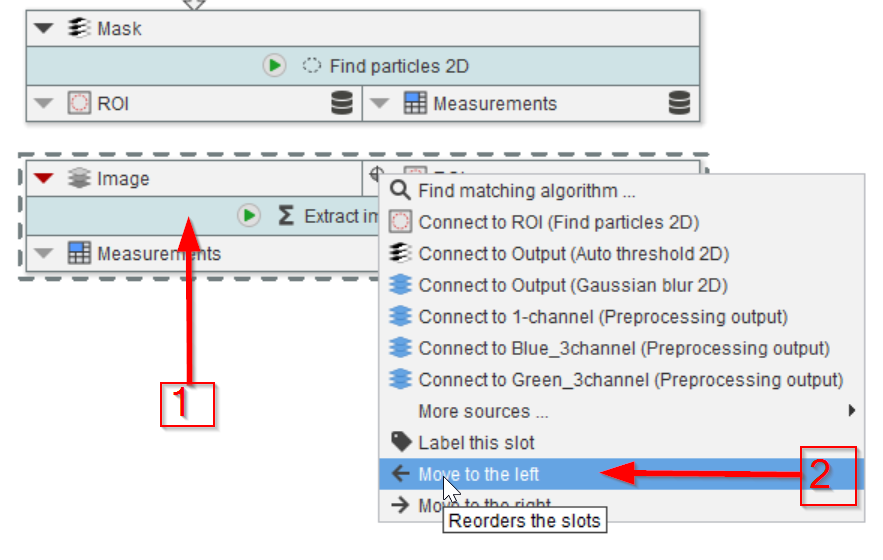
Step 4

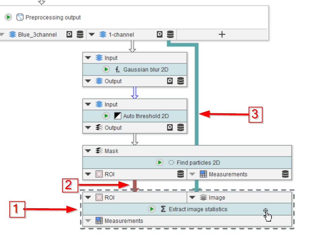
Drag the new node to the UI and position it below the Find particles 2D node (red arrow 1). For convenience, rearrange to input slots of the new node by moving its right-side node to the left (red arrow 2) by clicking the ▼ button on the ROI slot and selecting Move to the left.

Info

You can also right-click a slot to open the slot settings menu.

Step 5

Connect the node (red arrow 1) to the ROI output of the Find particles 2D node to get the list (red arrow 2).

Connect the Image input to the 1-channel output of the Preprocessing output node (red arrow 3).

Step 6

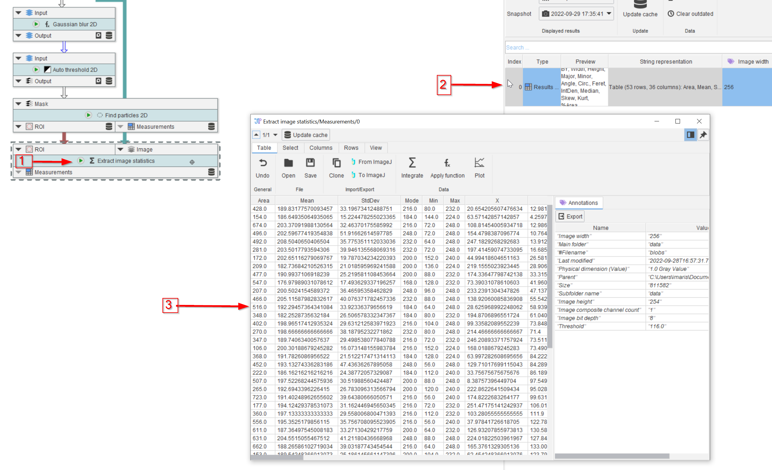
Run the node (red arrow 1) and observe the cached result (red arrow 2) in a viewer (red arrow 3).

Step 7

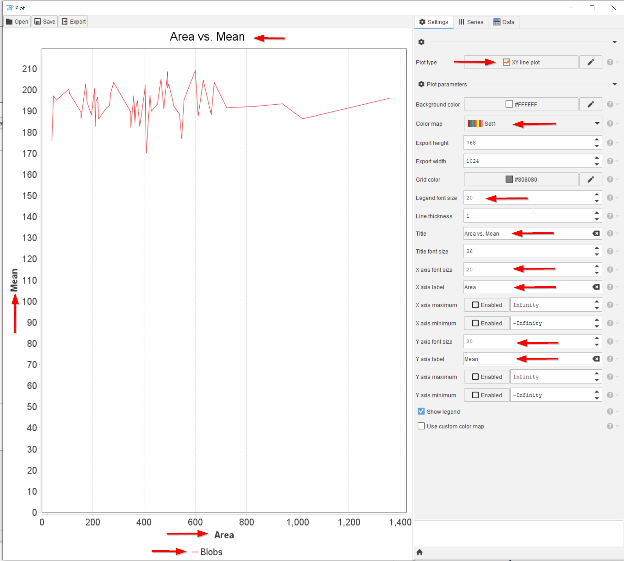
Plot the Mean values vs. the Area using the Table’s plot function, as shown in a tutorial before.

The red arrows show the settings that were changed from the default values view the plot window.

Step 8

From this plot it appears that areas below 150 and above 700 are rare. We can ignore these values by filtering the ROIs.

Look for such node via the top menu and navigate to ROI (red arrow 1), then Filter (red arrow 2), and choose Filter ROI by statistics (red arrow 3).

Info

Filter ROI by statistics allows to filter a ROI list via custom mathematical expressions. ImageJ measurements and annotations are both available.

Step 9

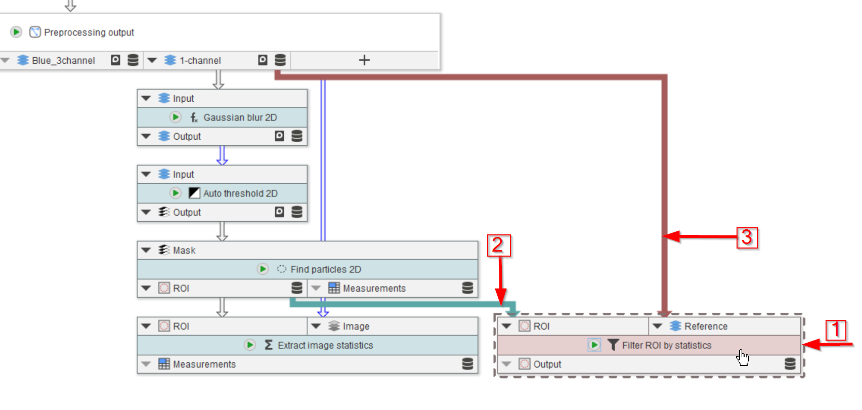
Add the node to the UI (red arrow 1) and connect it to the ROI output slot of Find particles (red arrow 2), and to the 1-channel output slot of the Preprocessing output node (red arrow 3).

Step 10

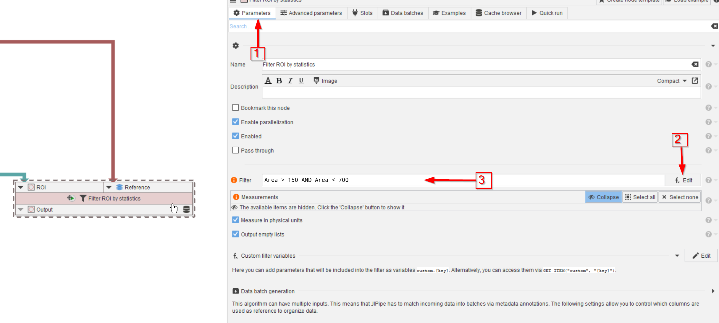
Go to the Parameters tab of the Filter ROI by statistics node (red arrow 1) and use the expression editor (red arrow 2) as shown before to create the filtering formula (red arrow 3):

Area > 150 AND Area < 700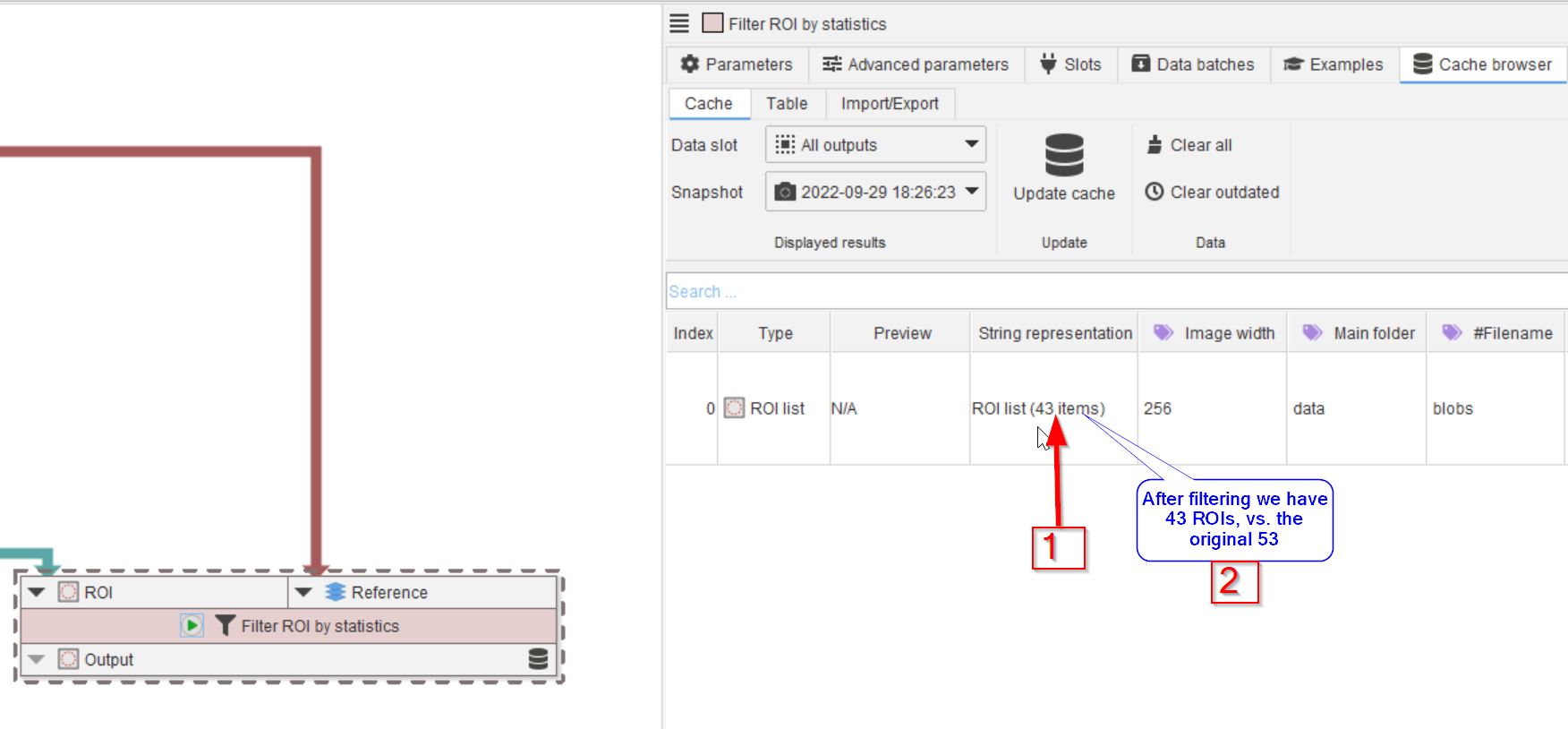

Tip

Here you do not need to write TO_NUMBER(Area), as the values are already numeric to begin with. Unlike text-based annotations that come from JIPipe’s data management functions, Filter ROI by statistics extracts its values from ImageJ tables that support numbers.
If you incorporate annotations into your formula, you then should use TO_NUMBER, e.g., TO_NUMBER(numChannels).

Step 11

Run the node and observe the lower number of ROIs (red arrow 1, note 2).

Step 12

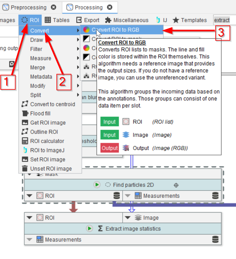
We now plot the selected ROIs in an overlay image with the original 1-channel data. Browse the ROI menu (red arrow 1) to look for Convert functions (red arrow 2), and select the Convert ROI to RGB function (red arrow 3).

Tip

Convert ROI to RGB visualizes ROI on top of an image. It is JIPipe’s equivalent of the ImageJ ROI Manager’s visualization feature.

Step 13

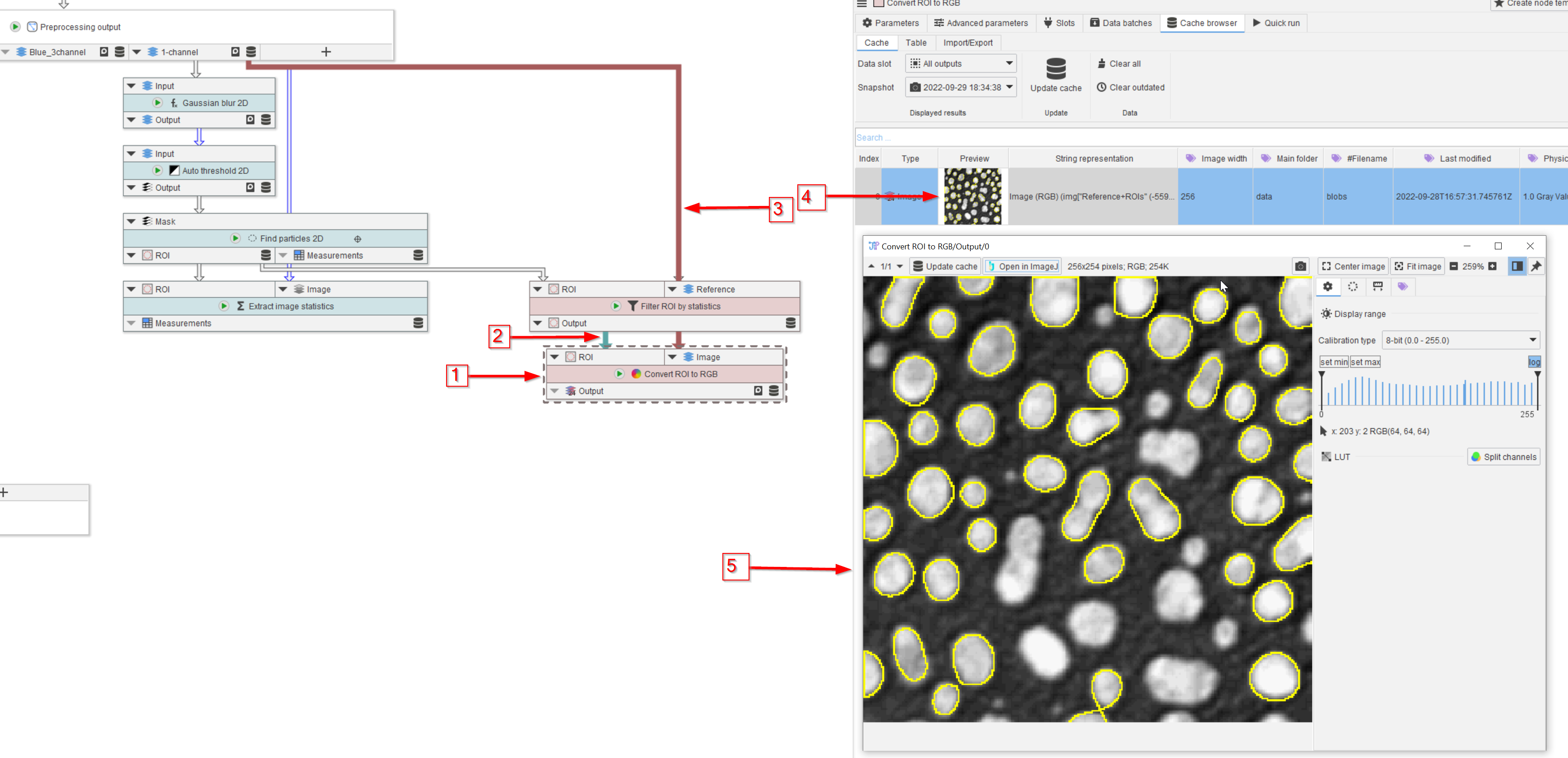
Add the node to the UI (red arrow 1), connect it to the filtered ROI list (red arrow 2) and to the 1-channel image (red arrow 3).

Run the node and observe the cache entry (red arrow 4) and the full image in a viewer (red arrow 5). The exclusion of the very small and very large ROIs can be observed.

Step 14

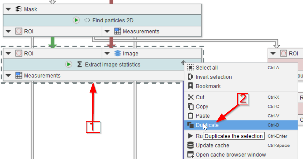
Select the image statistics node (red arrow 1) and duplicate it (red arrow 2). This menu is accessible via right-clicking on the middle green area of the node.

Step 15

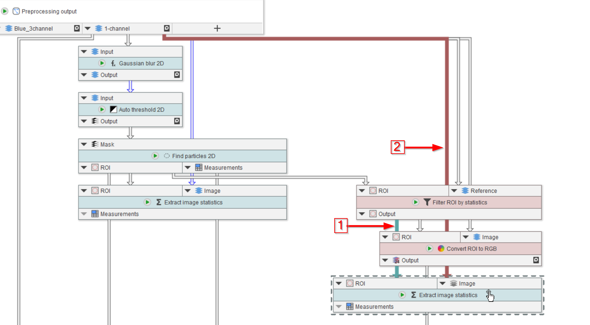
Connect the duplicated node to the filtered ROI output (red arrow 1) and to the 1-channel image (red arrow 2).

Create two new input nodes on the Processing compartment output node: one for the filtered ROI measurements, and one for the ROI overlay image.

Connect the old output slots (red arrows 1-3), as well as the two new ones to the output node (red arrow 4-5).

Now the statistics are extracted from filtered ROIs.