
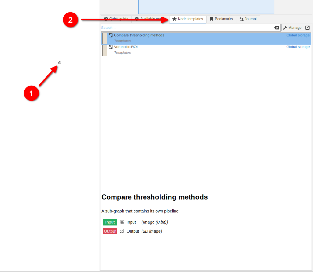


Preliminary steps
👉 This tutorial requires that you have installed node template Import images.
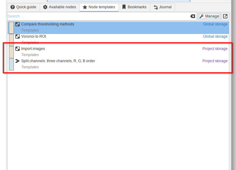
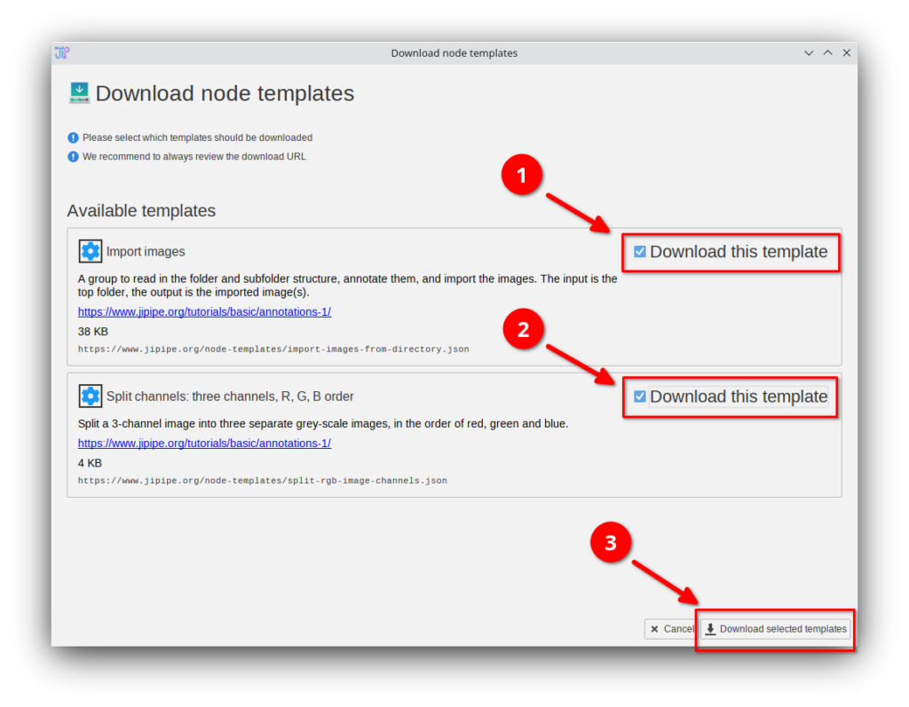
If you do not have these templates, you can download them via Manage > Download more templates or by importing the Templates.json file that is provided in the data package. If you do not know how to download or import node templates, please check out our tutorial.

Step 1
Load a 1-compartment template into JIPipe and add the data folder of the tutorial to the UI (red arrow 1).
Drag the Import images template node from the Node templates list to the UI and connect it to the Folders node (red arrows 2). Run this node and observe that cache browser (red arrow 3) that now shows 20 images of the droplet example (red rectangle 4).
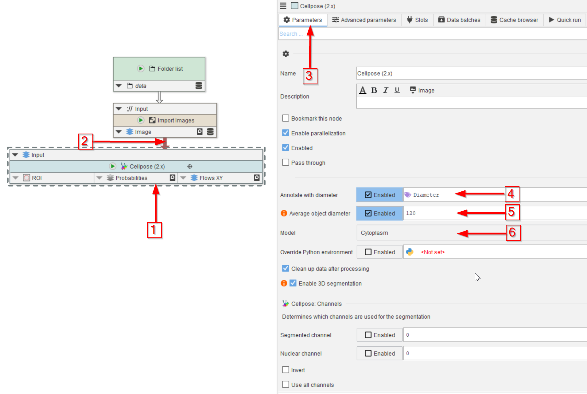
Step 2
Add a Cellpose (2.x) node to the UI (red arrow 1) and connect it to the Import images node (red arrow 2).
In the Parameters tab (red arrow 3) observe the default annotation Diameter (which is the size guidance for the objects to be found; red arrow 4) and set the Average object diameter parameter to Enabled and its value to 120 (red arrow 5).
Set the segmentation model to Cytoplasm (red arrow 6), which is one of the pre-trained models of Cellpose, and it should work well with the general circular shape of the droplets.
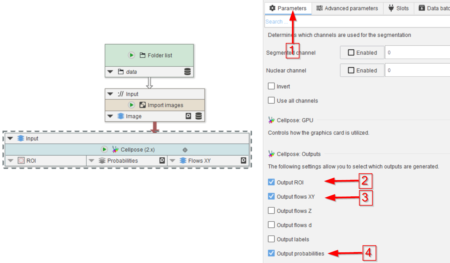
Step 3
Still in Parameters (red arrow 1), select the outputs of your choice.
In this example, we will chose the segmented areas as ROIs (red arrow 2), the flows (red arrow 3), and the probability map (red arrow 4).
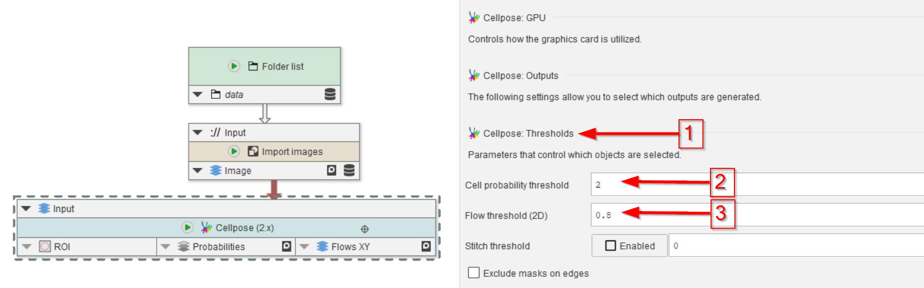
Step 4
The flow and probability maps are thresholded before the segmented ROIs are generated.
These threshold values can be set in the corresponding menu (red arrow 1), where the probability threshold (red arrow 2) and the flow threshold (red arrow 3) can be set.

Step 5
Guidance for these levels can be gained from examining the probability map and identifying the typical levels at the image features of interest.
In the Cache browser (red arrow 1) choose the Probabilities data slot (red arrow 2) and examine the outcome (red rectangle 3). Open an item of interest by double-clicking it and use the mouse pointer to observe the values.

Step 6
By examining the ROI output, it is evident that the results need to be filtered in order to select the round main object.

Step 7
This task will be carried out by adding a Filter ROI by statistics node (red arrow 1), connecting it to the ROI output of the Cellpose (2.x) node (red arrow 2), and setting the roundness threshold to 0.7 (red arrow 3):
Round > 0.7
Step 8
We will now shape the identified droplet ROI by converting the ROIs to a mask (red arrow 1) by applying a Morphological operation 2D (red arrow 2) to open the object (red arrow 3) with a Radius of 10 px (red arrow 4), using a Disk-shaped kernel (red arrow 5).
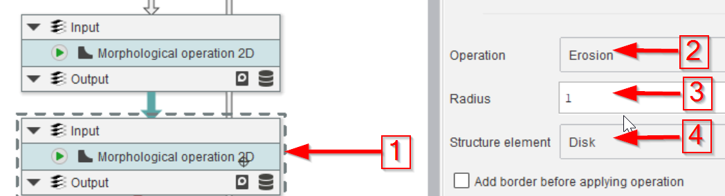
Step 9
The next Morphological operation 2D (red arrow 1) will implement an erosion (red arrow 2) with a 1-pixel (red arrow 3) disk kernel (red arrow 4).
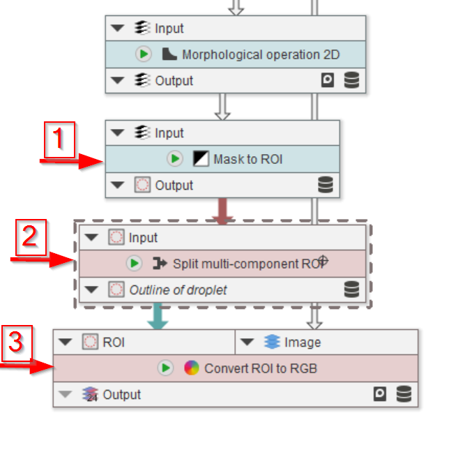
Step 10
The last three nodes will convert the mask back to ROIs (red arrow 1), split them in case more than one full droplet is found (red arrow 2), and show the quality of the segmentation by overlaying the ROIs with the image (red arrow 3).

Step 11
Here the Image input slot (red arrow 2) of the Convert ROI to RGB node (red arrow 1) is connected to the Image output of the Import images node (red arrow 3).