Table processing
Illustrates how to use some table processing capabilities included in JIPipe
Tutorial: Table processing
Step 1
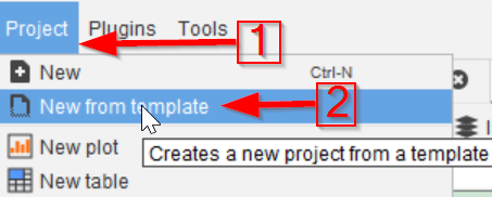
Create a new JIPipe project (red arrow 1) using a template (red arrow 2).
Step 2
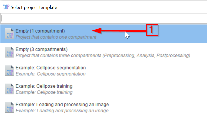
Create a new JIPipe project (red arrow 1) using a template (red arrow 2).
Step 3
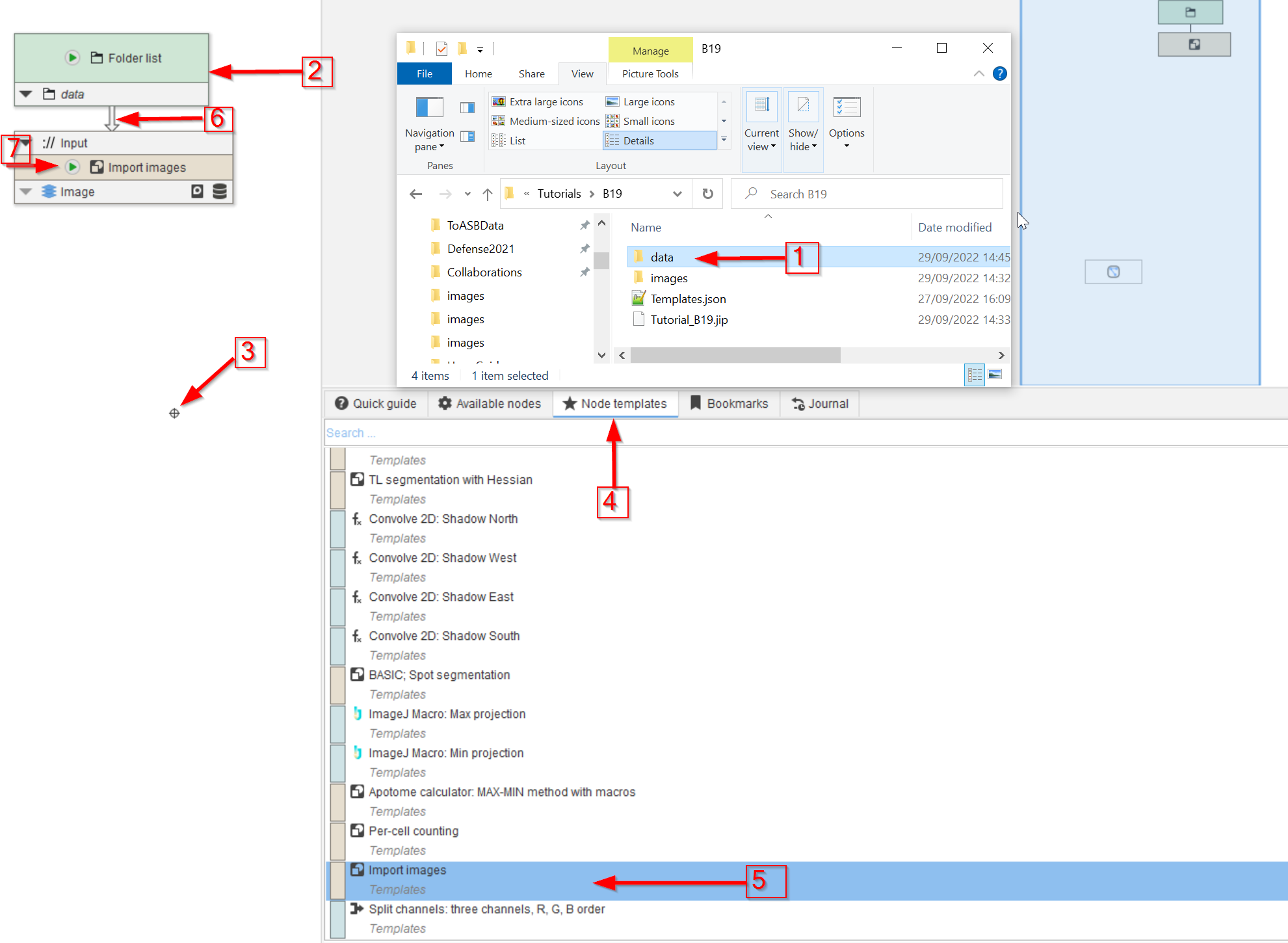
Locate the data folder that belongs to this tutorial (red arrow 1) and drop it on the UI (red arrow 2).
Click somewhere on the white area of the UI (red arrow 3) and chose the Node templates tab (red arrow 4).
👉 This tutorial requires that you have installed node template Import images.
If you do not have the template, you can download it via Manage > Download more templates or by importing the Templates.json file that is provided in the data package. If you do not know how to download or import node templates, please check out our tutorial.
Select the pre-made Import images template from the list (red arrow 5) and drag it to the UI. Connect it to the Folder list node (red arrow 6) and run the Import images node (red arrow 7.)
Step 4
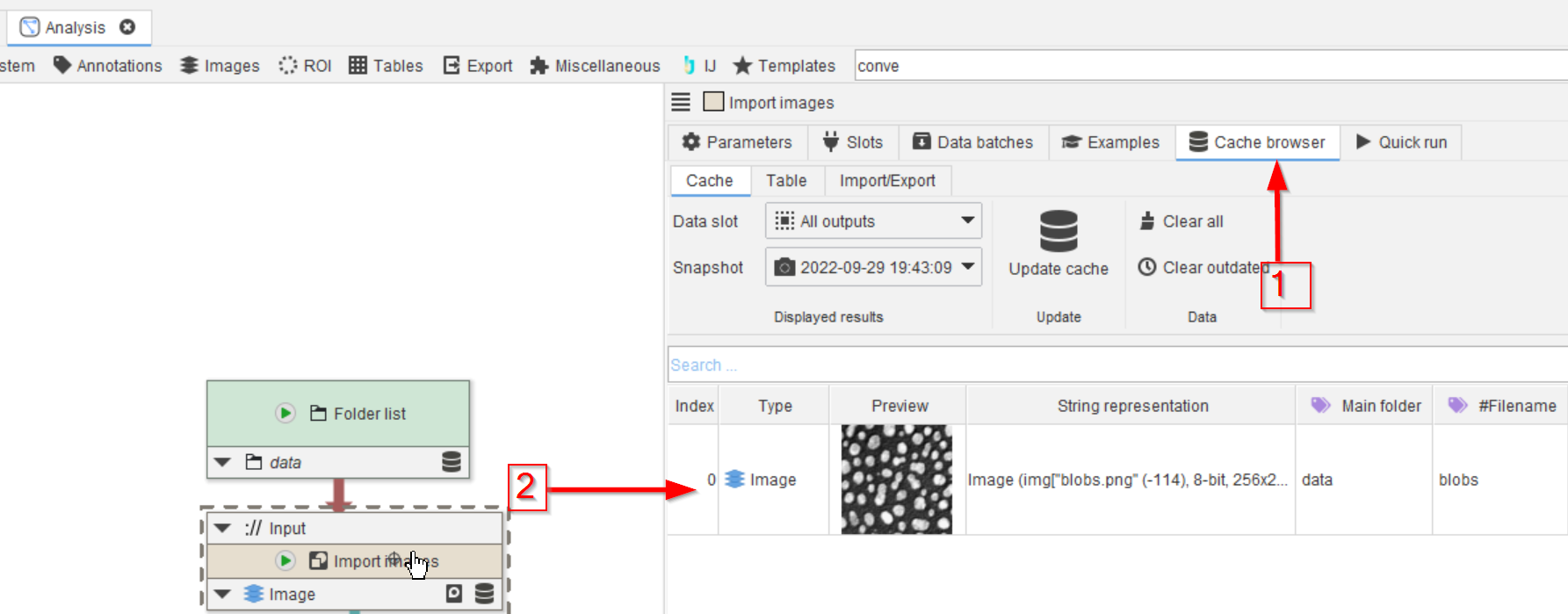
The Cache browser (red arrow 1) will now show the fluorescence image (red arrow 2).
Step 5
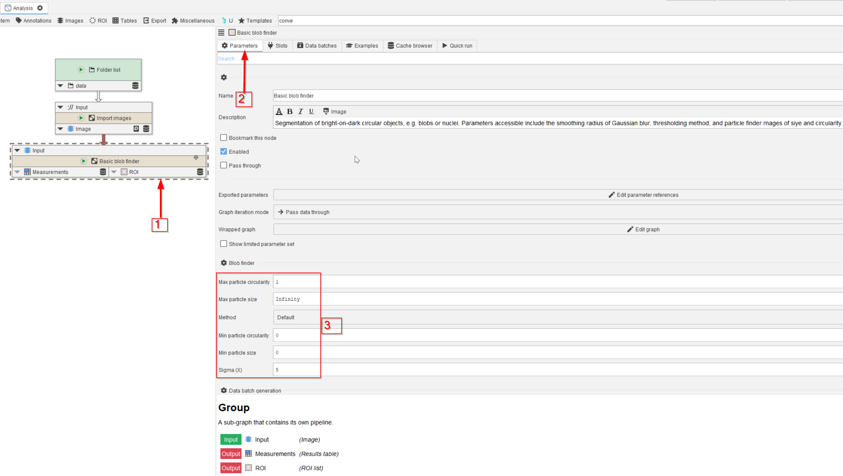
Add the Basic blob finder template to the UI (red arrow 1) and observe the Parameters tab (red arrow 2).
The exposed parameter of the group node are indicated here (red rectangle 3), including the particle size and circularity ranges, the thresholding method and the gaussian smoothing factor.
Step 6
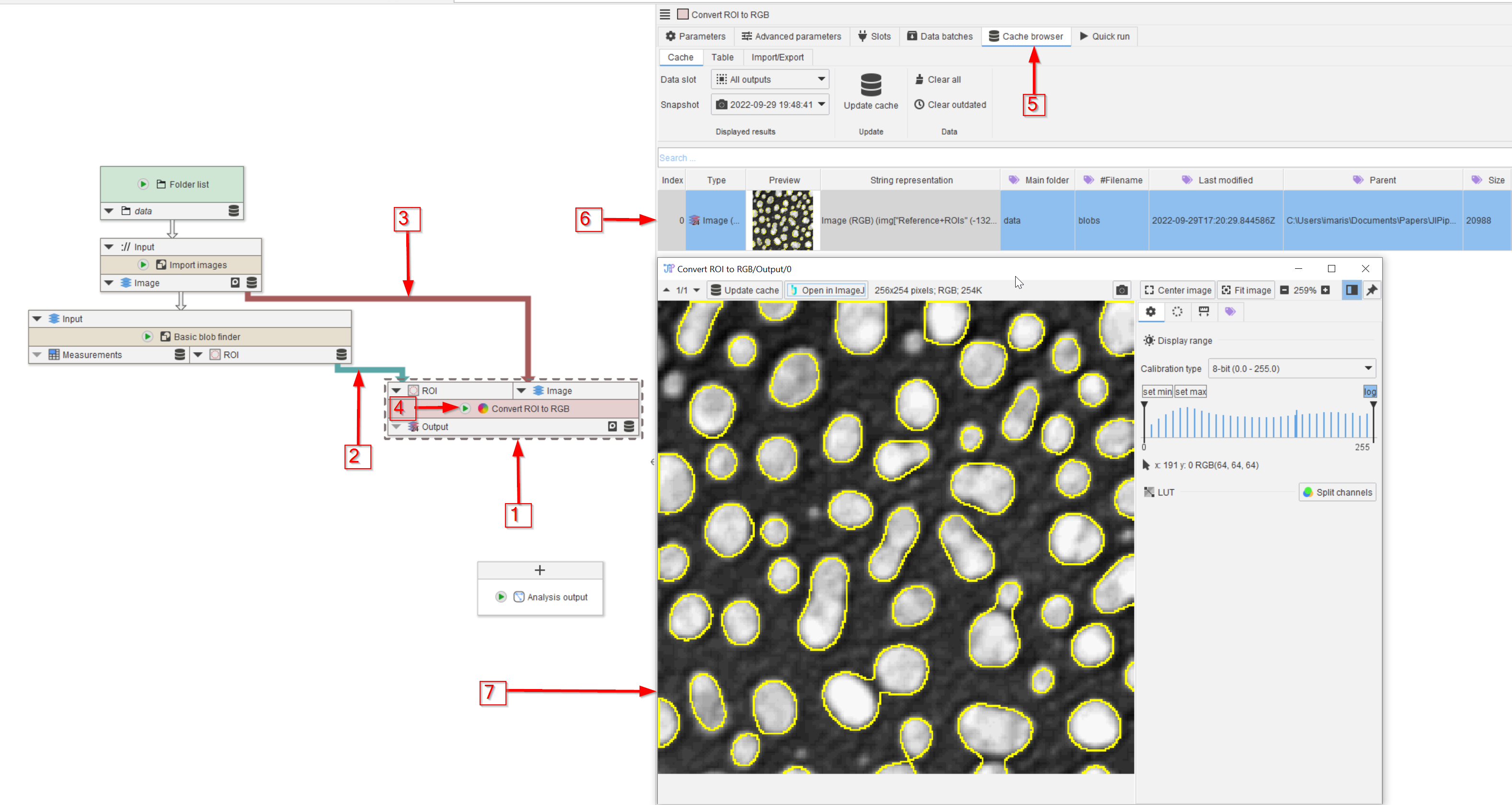
In order to observe the quality of the segmentation, add a Convert ROI to RGB node (red arrow 1), connect it to the ROI and Image outputs of the Import images and Basic blob finder nodes (red arrows 2 and 3), and run it (red arrow 4).
In the Cache browser (red arrow 5), observe the entry (red arrow 6) and the full image (red arrow 7).
Step 7
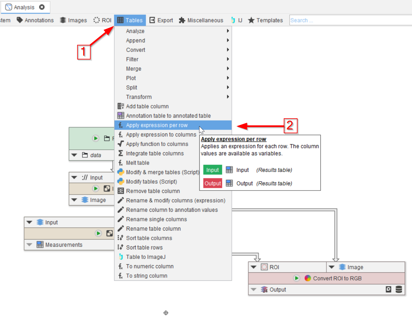
Look for Table processing nodes in the Tables menu (red arrow 1) and select the node Apply expression per row (red arrow 2).
Connect the node to the Measurements output of the Simple blob finder.
The Apply expression per row node applies a custom mathematical expression for each row of the input table. The result of the expression is written into a new or existing column of the same row.
The mathematical expression has access to the annotations of the incoming table, as well as the values of each column within the same row.
Step 8
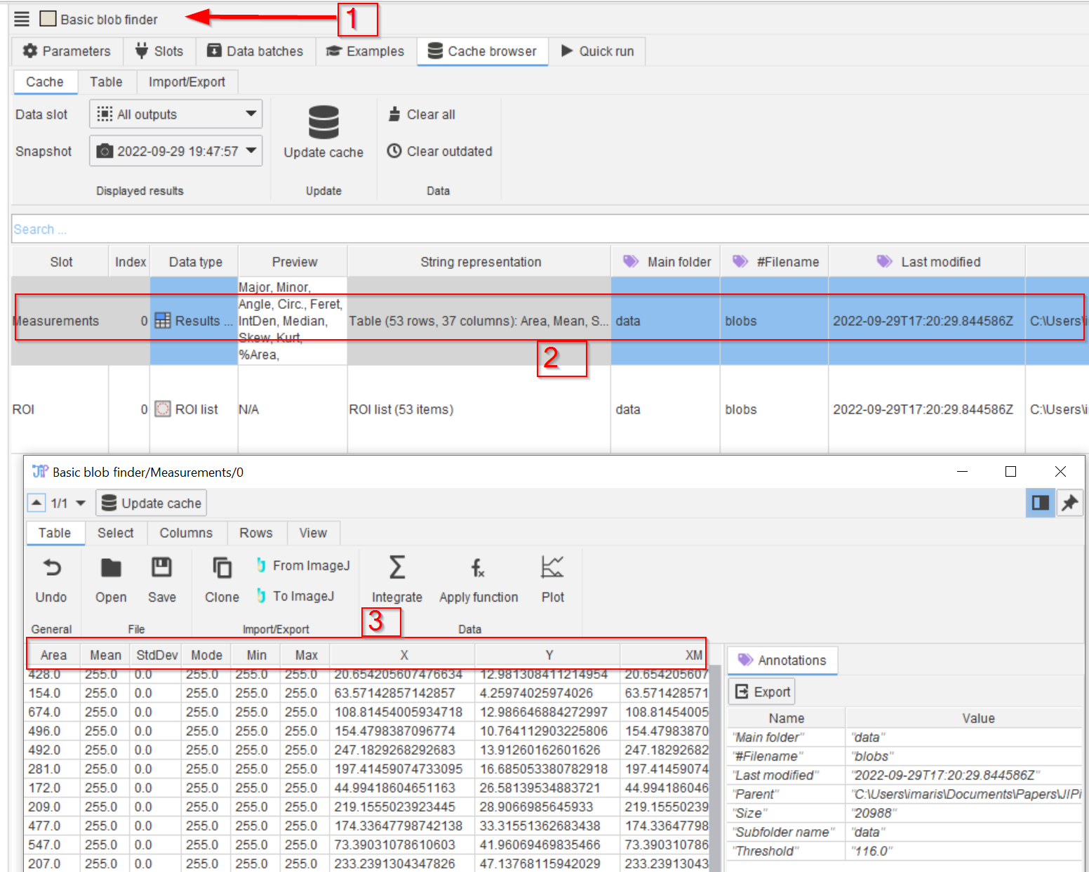
Before editing the table, find out the names of the measured parameters:
open the Measurements cache results of the Basic blob finder (red arrow 1), double-click on the cache entry (rectangle 2) and review the column names in the table viewer (rectangle 3).
Step 9
Let us calculate the ratio between the mean value and the area.
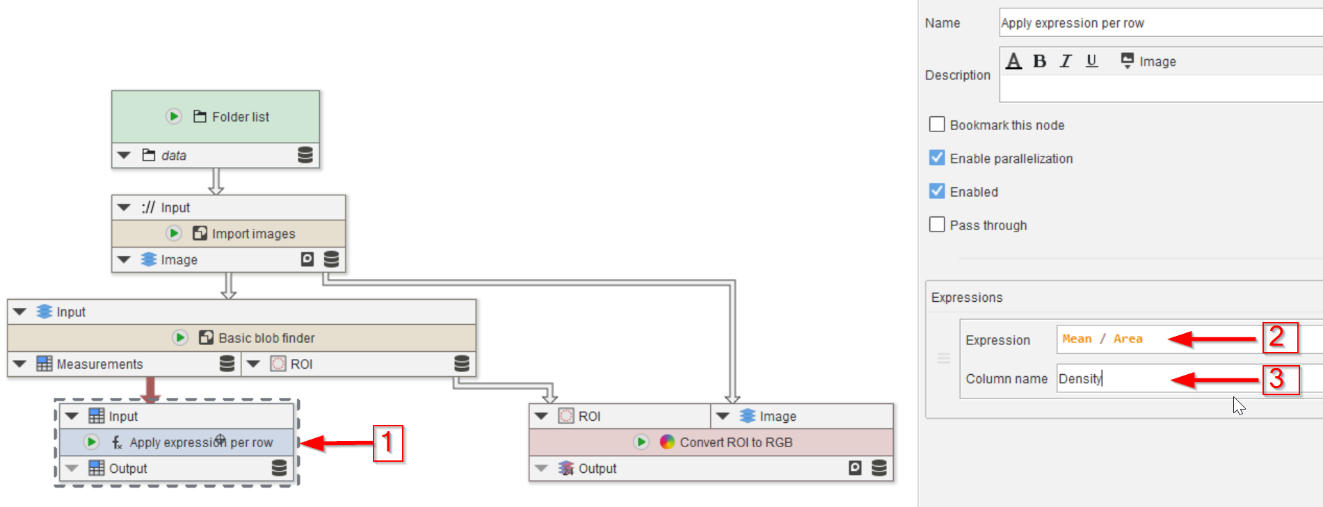
Select the Apply expression per row node (red arrow 1), open the Parameters tab and apply the following changes:
In parameter Expressions set the value of Expression to Mean / Area.
Mean and Area reference the mean and area column values of the currently processed row. Always keep in mind that the Expression is applied per row.
In parameter Expressions set the value of Column name to Density.
The meaning of this instruction is that the calculated result of Mean / Area will be written into a column Density in the output table.
If the column does not exist, the node will automatically create a new one.
Step 10
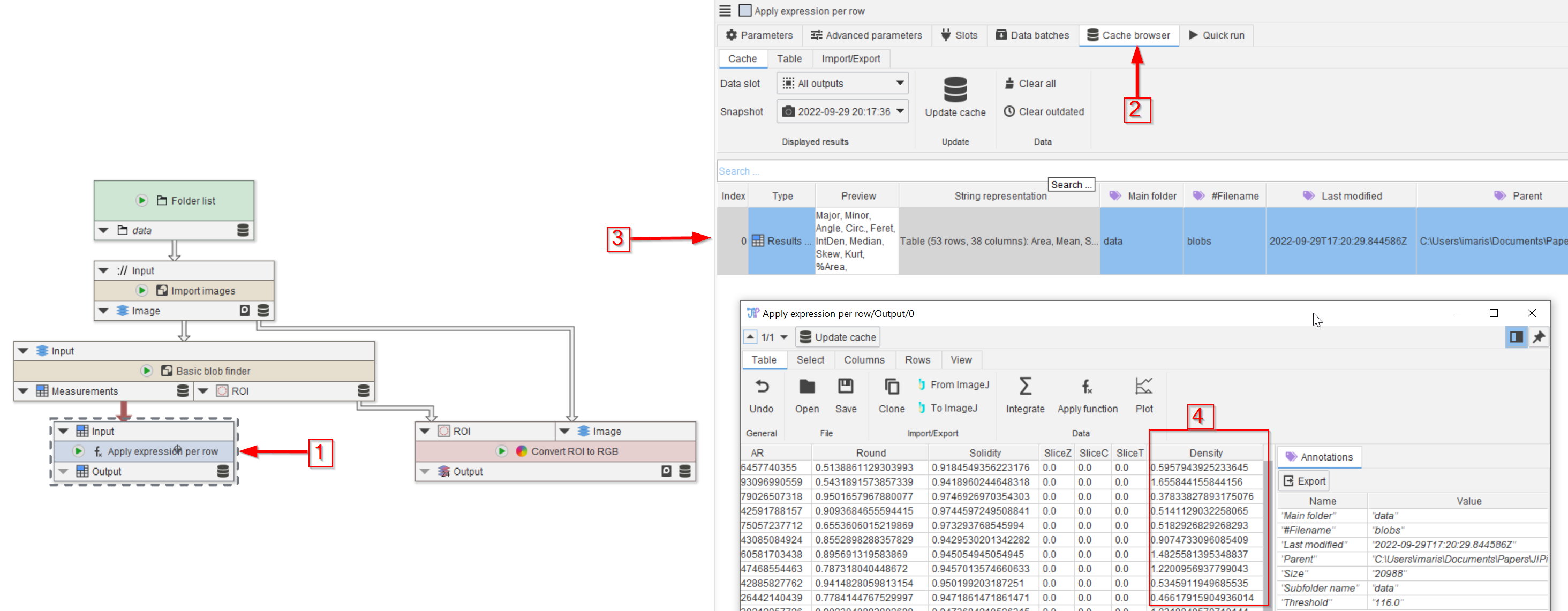
Run the node (red arrow 1) and observe the Cache browser (red arrow 2).
The cache entry (red arrow 3) now contains a new Density column (red arrow 4).
Step 11
We will proceed to generate an integrated table.
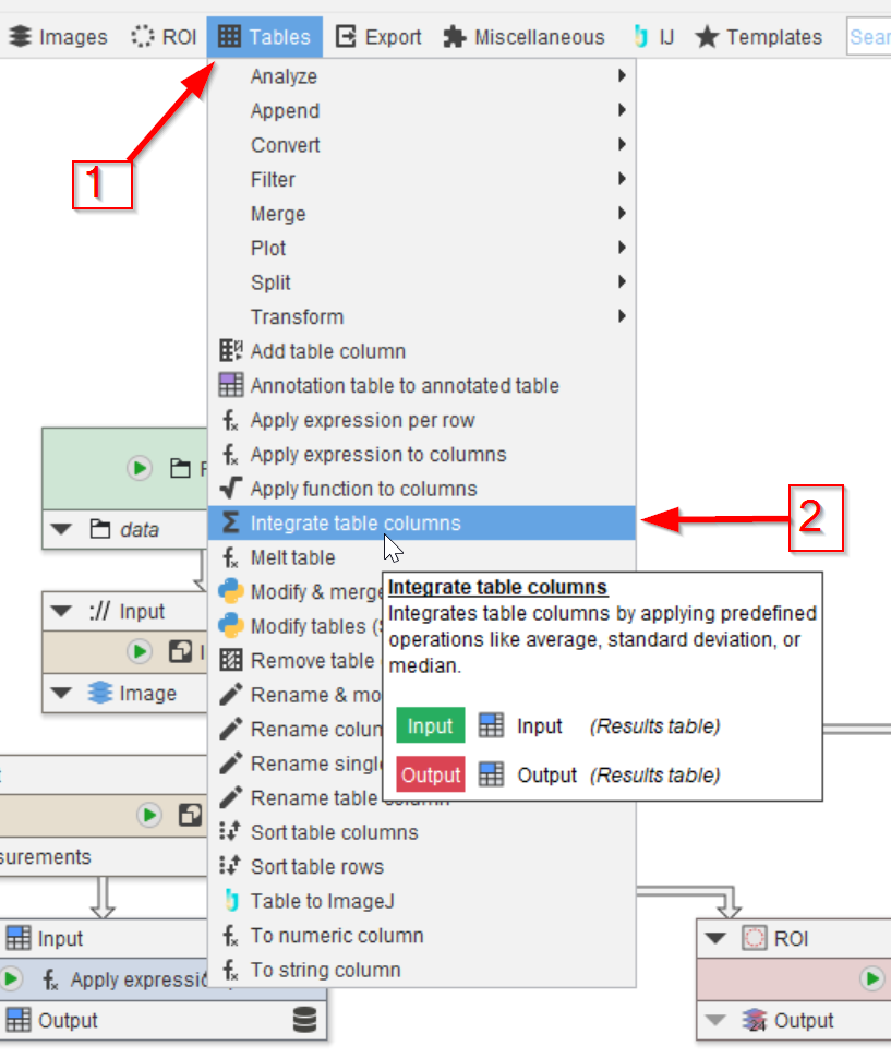
From the Tables menu (red arrow 1), add the node Integrate table columns (red arrow 2).
Integrate table columns allows to apply pre-defined integration methods (sum, min, max, mean, first or last row, …) to a customizable set of table columns.
The result will be a table with one row.
If you want to write a custom integration function, use Apply expression to columns that utilizes mathematical expressions.
Step 12
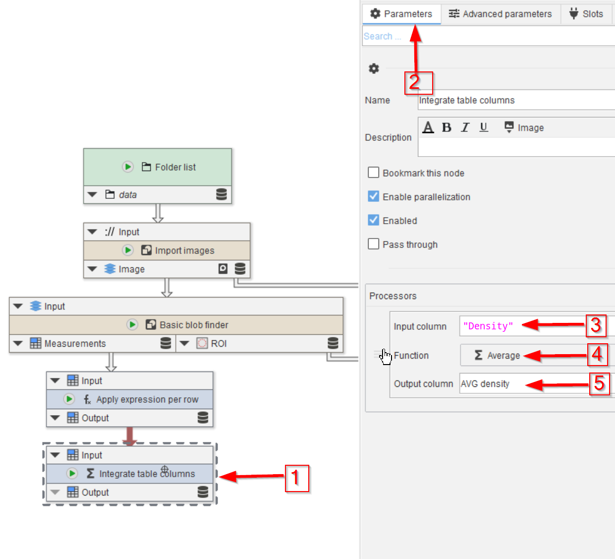
Select the Integrate table columns (red arrow 1) and edit the Processors parameters in the Parameters tab (red arrow 2):
Set the Input column to the following value:
"Density"
If you reference existing columns, always put the name in quotation marks. The function for selecting columns can be heavily customized, as it is expression-based an can under certain circumstances yield unexpected results if the name is typed in as is.
For example, if there is an annotation Density set to XYZ, and the expression is just set to Density, the node would search for a column with the name XYZ, as the expression system tries to look for a known value with the name Density.
This will not happen if you put quotation marks around the column name, e.g., "Density".
Proceed by choosing the Average as a mode of operation (red arrow 4), and provide a name for the new results (e.g., AVG density, red arrow 5).
The Output column does not require quotation marks, as it is not an expression - just a text.
You can differentiate expressions from text by the UI design:
- Expressions are colored, while pure text is always black
- Expressions have an Edit button, while pure text has a button to clear the current value.
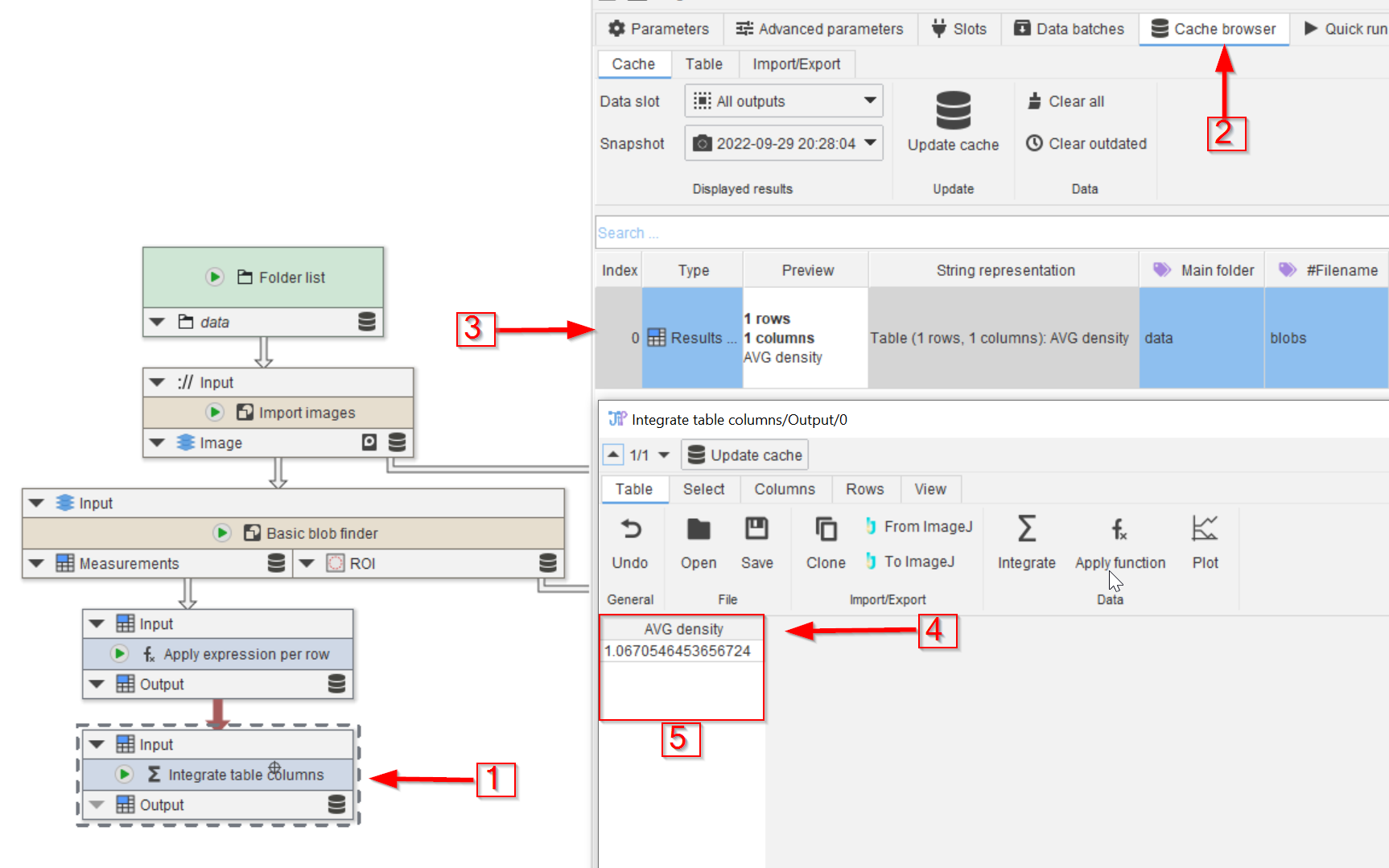
Step 13
Run the node (red arrow 1) and observe the Cache (red arrow 2).
The new cache entry (red arrow 3) now contains the new column AVG density (red arrow 4, red rectangle 5).
If you want to annotate data (an image, table, etc.) by the AVG density, use the node Annotate data with table values.
Its Generated annotation parameter allows to generate an annotation from value(s) obtained from a table and attach it to the input of the Data slot.
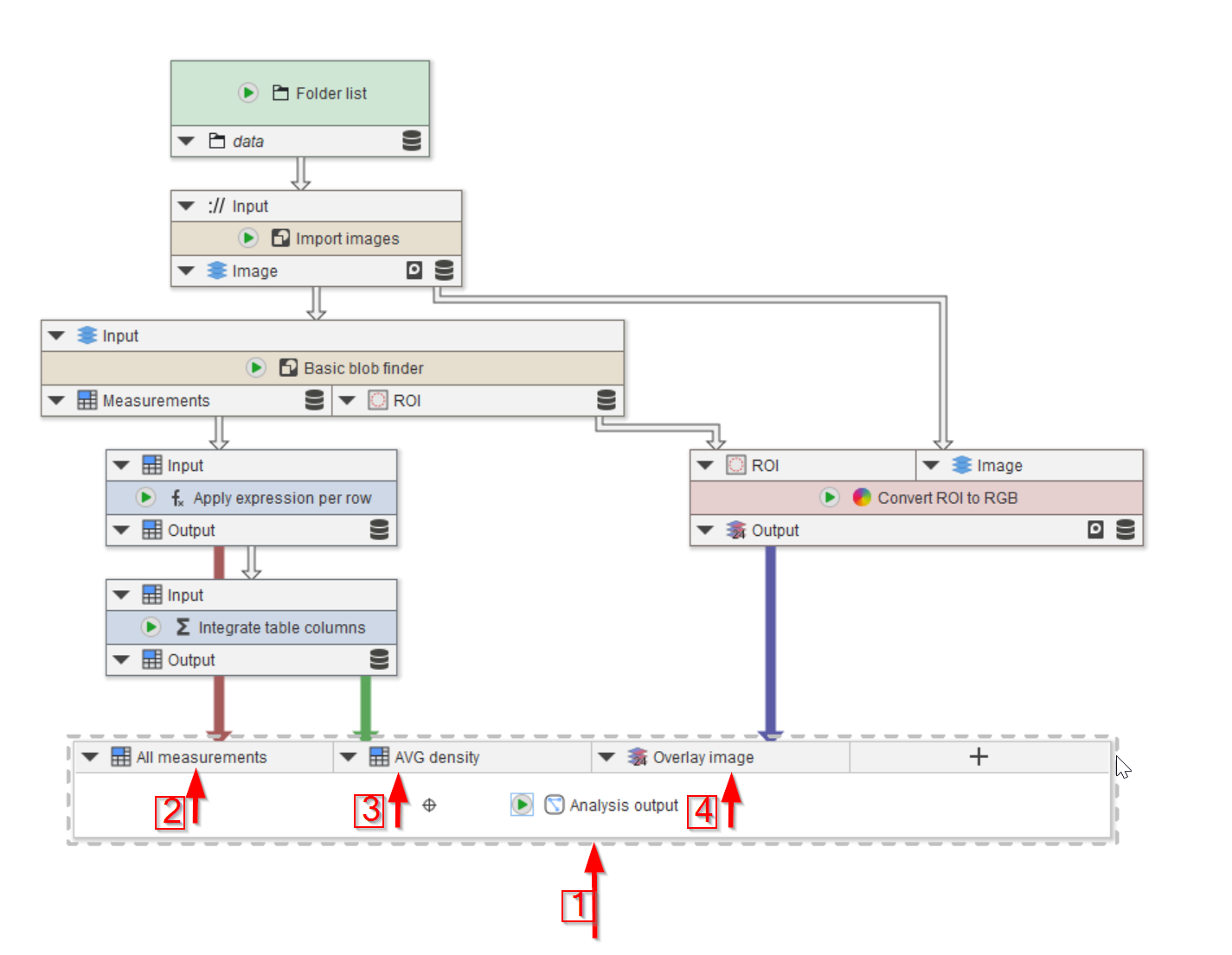
Step 14
Finally, add three input nodes to the compartment’s output node and connect them accordingly. (red arrows 1-3).