Compartments II: Basic image segmentation
Explains how to apply basic image segmentation on a compartmentalized pipeline
Tutorial: Compartments I (Creating and connecting)
Step 1
Please ensure that you have followed the tutorial Compartments I: Creating and connecting
Navigate to the Processing compartment.
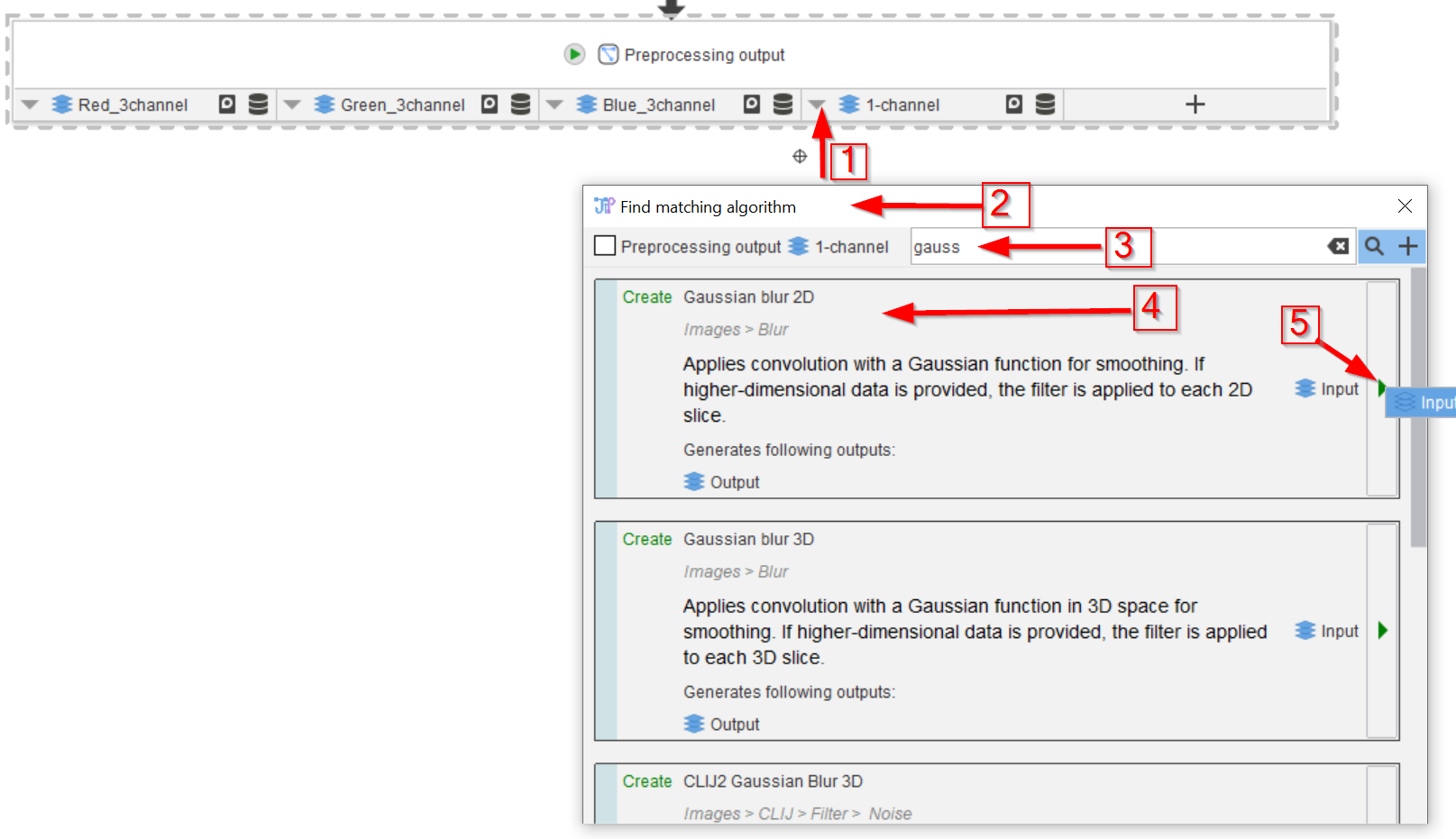
We start with segmenting the blob image. We can use the node search triangle (red arrow 1) to find matching nodes (red arrow 2). Search for gaussian blur (red arrow 3) and select the Gaussian blur 2D node (red arrow 4).
Add the node to the pipeline (red arrow 5).
Step 2
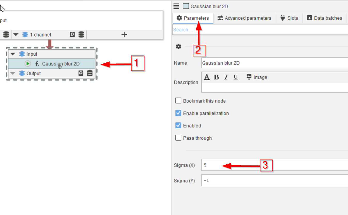
Select the newly added node (red arrow 1) and go to Parameter (red arrow 2).
Experiment with the node by setting the Sigma (X) parameter (red arrow 3) to various value by running the node and examining the cache content.
Step 3
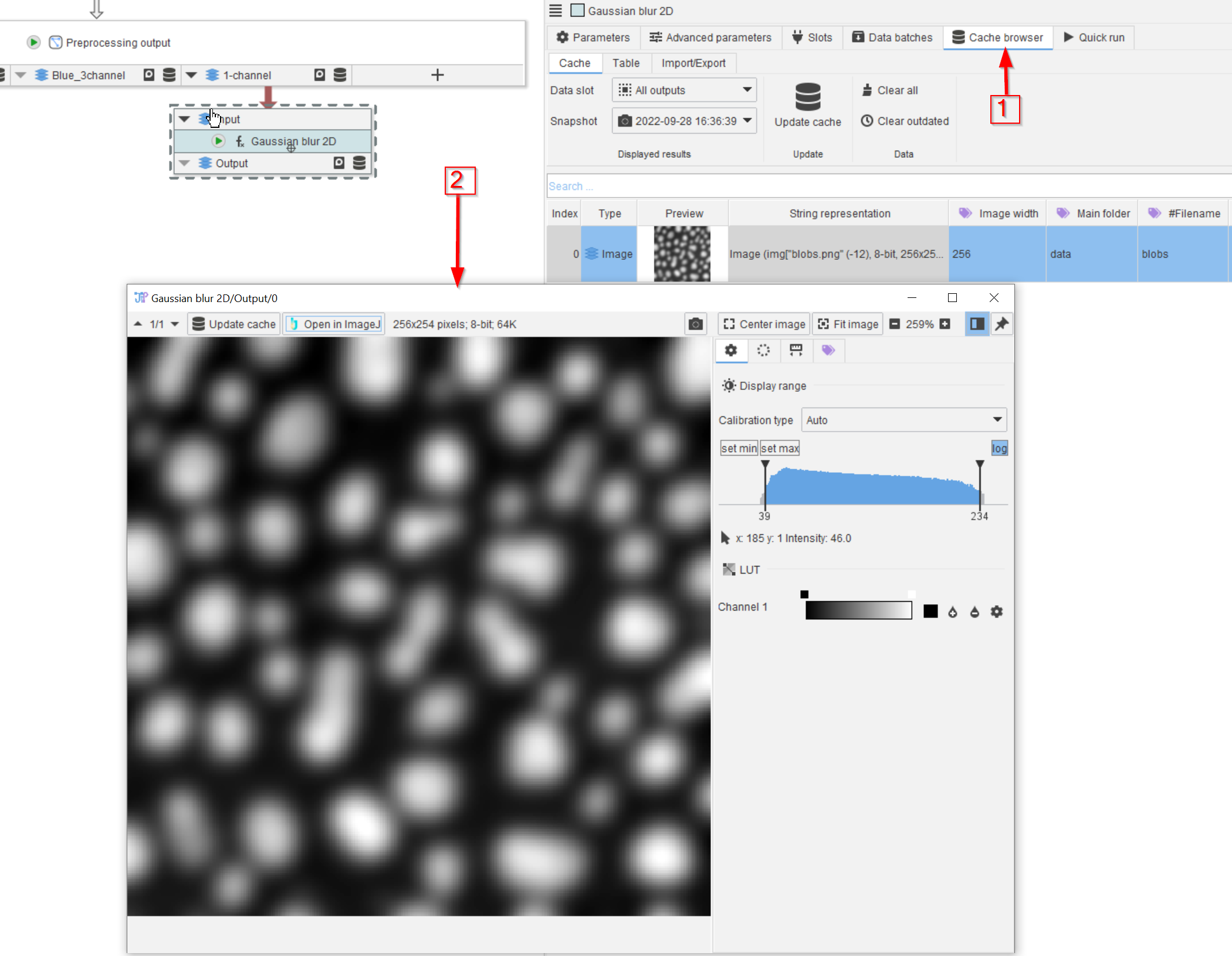
With Sigma set to 5, the cache (red arrow 1) should show a blurred image as shown below (red arrow 2).
Step 4
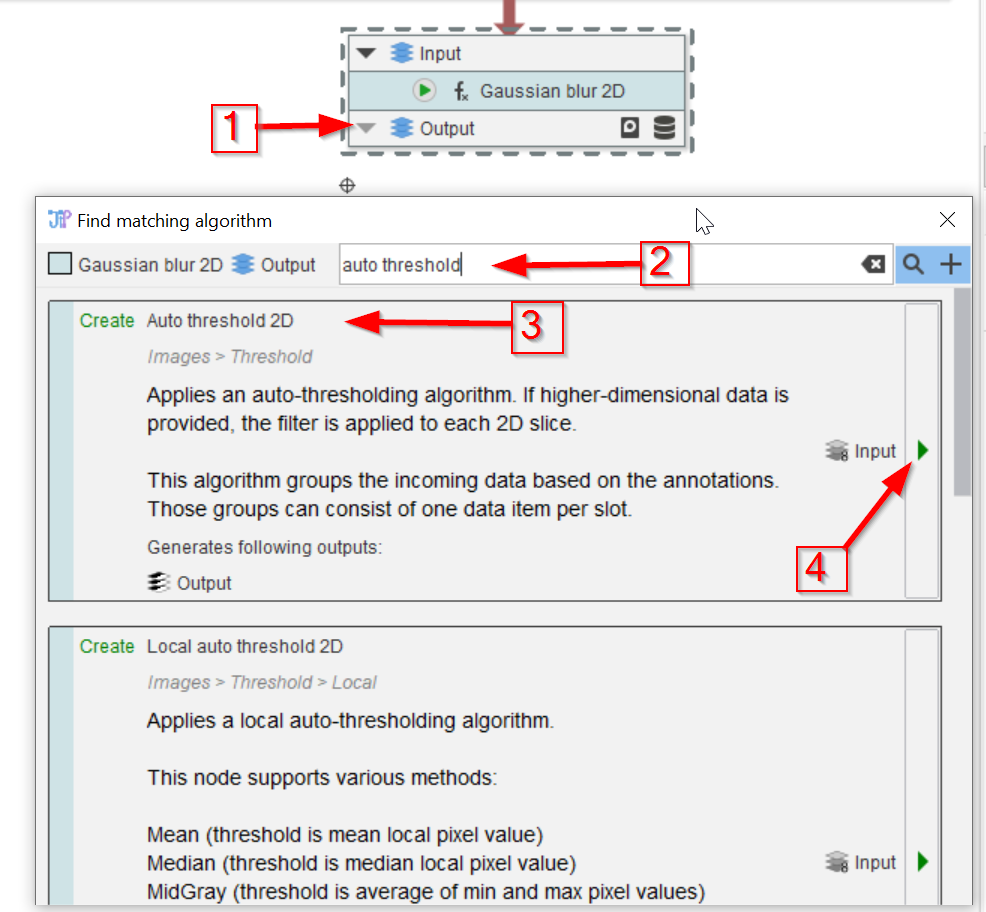
A simple segmentation can achieved by automatic thresholding. We search for such node e.g., via the Find matching algorithms option (red arrow 1) and searching for auto threshold (red arrow 2). Choose the matching node (Auto threshold 2D, red arrow 3) and add it to the pipeline (red arrow 4).
The Auto threshold 2D node is the JIPipe equivalent of the ImageJ command Image > Adjust > Auto threshold.
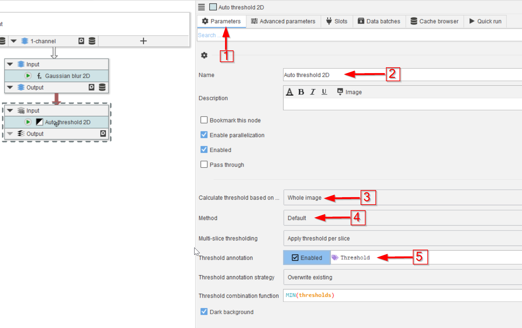
Step 5
The Parameters tab (red arrow 1) exposes the settings, the most important of which (for this tutorial) are indicated by the red arrow 2 to 5:
Calculate threshold based on ...allows to determine a ROI/mask from where the image threshold is calculated from (defaults to whole image)Methoddetermines the thresholding algorithm (defaults to ImageJ’s default thresholding)Threshold annotationdetermines if generated masks should be annotated with the calculated threshold value (defaults to an annotationThreshold)
Step 6
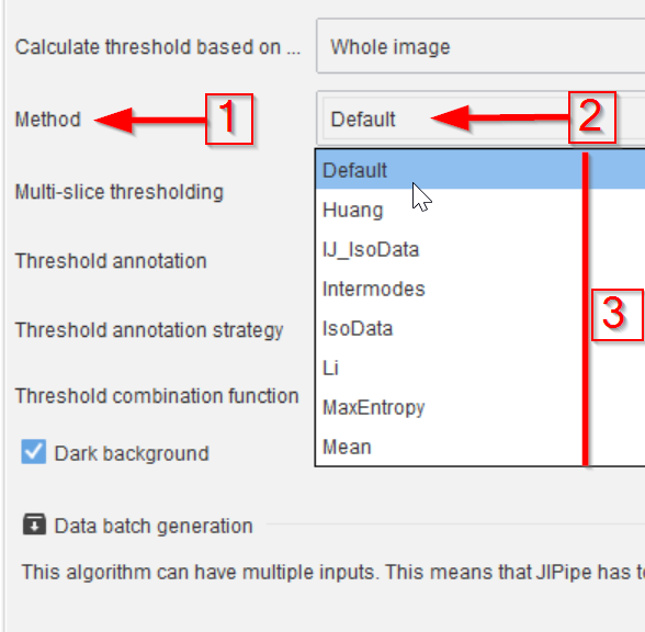
The most important parameter to test is the thresholding method (Method, red arrow 1), which is set to Default (red arrow 2) when creating a new node.
The menu allows to choose from the wide range of ImageJ-based methods (red line 3).
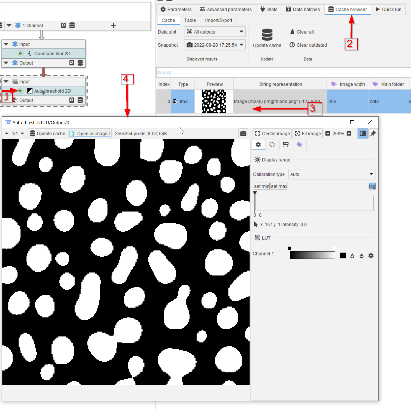
Step 7
Run the Auto threshold 2D node (red arrow 1) and observe the Cache browser (red arrow 2), where the thresholded image is now shown (red arrow 3). After double-clicking the cache entry (red arrow 3), the image viewer (red arrow 4) allows to display the binary image.
Step 8
The result is adequate, and it can be linked to the Processing compartment output.
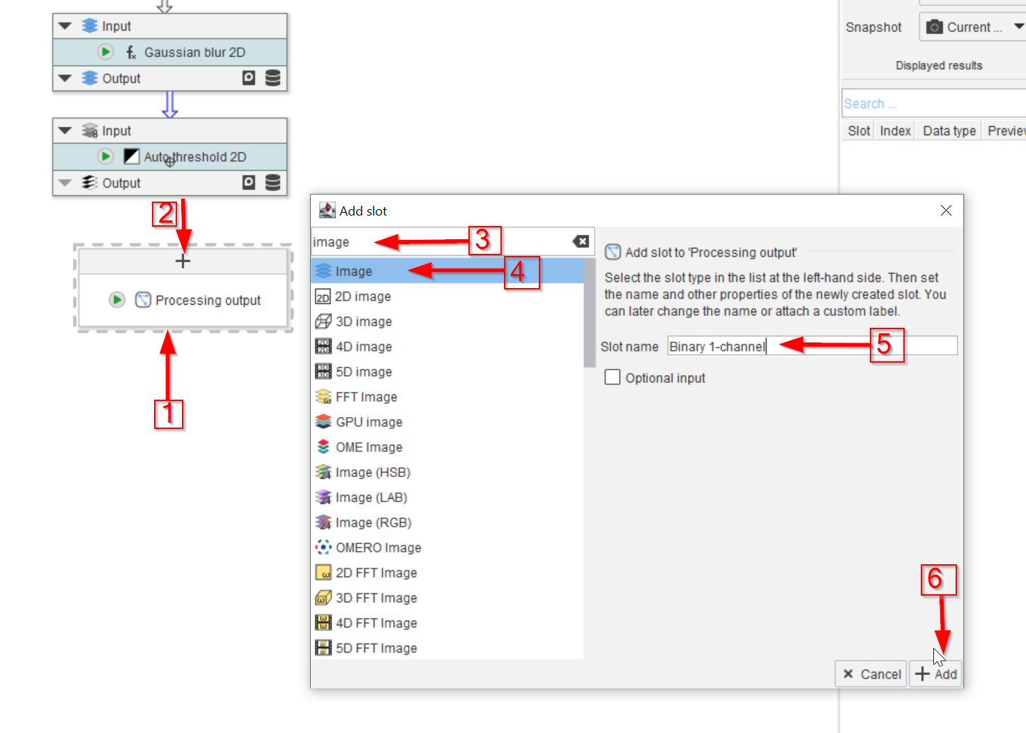
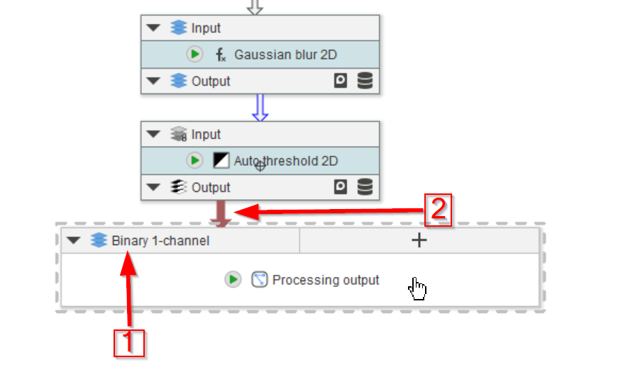
Locate the Processing output node and move it close to the thresholding node (red arrow 1).
Add a new input slot to the output node (red arrow 2) by searching for image in the search bar (red arrow 3) and selecting the general Image type (red arrow 4). Name the slot Binary 1-channel or any other name of your liking (red arrow 5) and add it to the node (red arrow 6).
Step 9
The new input slot is now available on the output node (red arrow 1). Connect it to the output slot of the thresholding node to expose the binary image as output of this node.