Cache I: Generating and viewing
Illustrates how to cache node results to the memory and how to browse through the generated data
Tutorial: Cache I (Generating and viewing)

Step 1
Load the example pipeline.
Go to the Compartments tab and update the cache directly from there. This can be achieved with the compartment nodes the same way as with regular nodes. Use the green arrow on the Processing compartment (red arrow 1) and choose the Cache intermediate results option to save the cache for all nodes (red arrow 2).
Note that the method of updating the cache from the compartments works only if the output node of the compartment is connected! See the previous tutorials on setting up the output nodes of compartments.
Step 2
The same cache options are of course available directly from inside the Processing node.
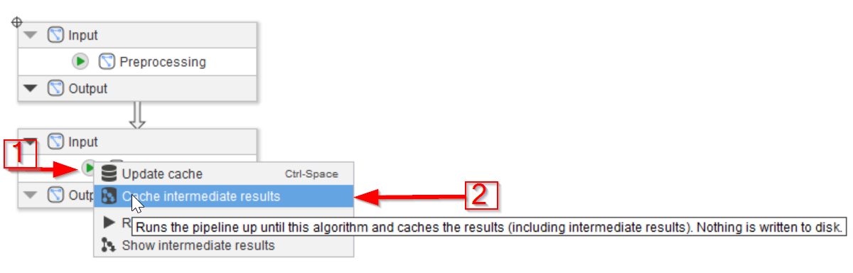
To run all the nodes and save their results in cache, use the green arrow in the bottom-most node (Processing output, red arrow 1) and choose the Cache intermediate results option (red arrow 2).
Step 3
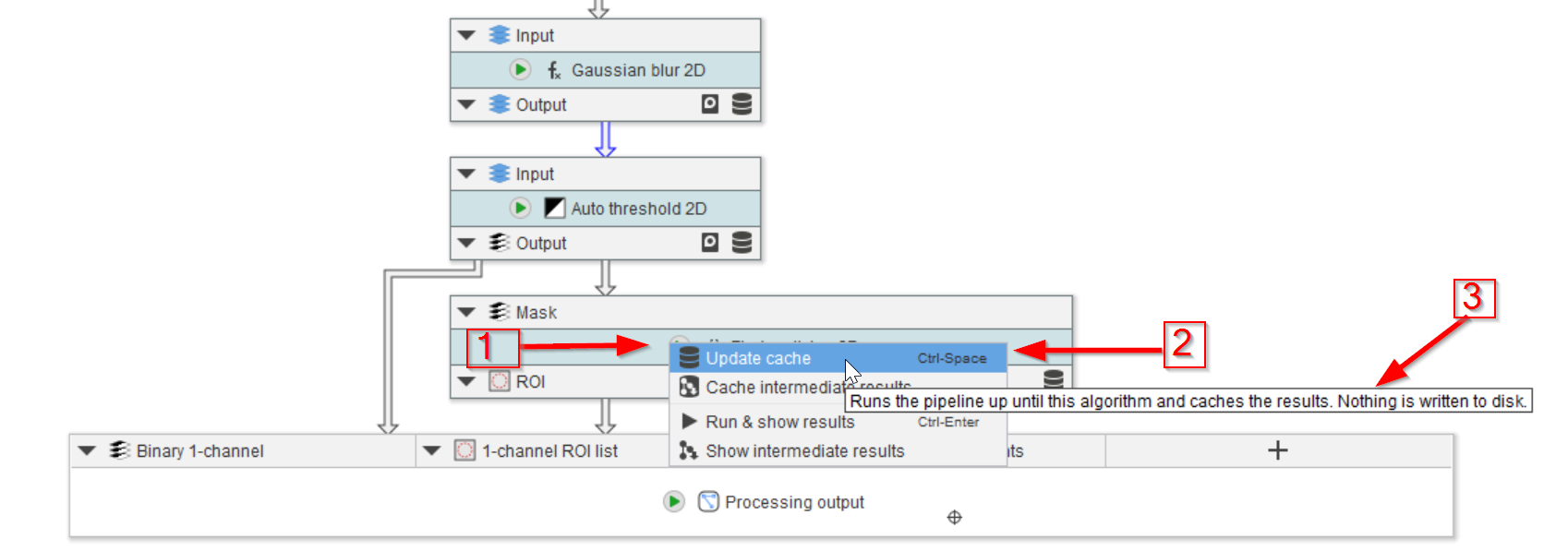
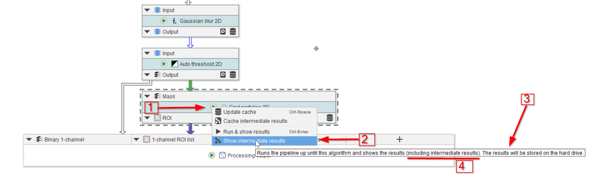
When only the last node’s cache needs to be updated, e.g., after changing parameter(s) only in that node (red arrow 1), the option of Update cache can be used (red arrow 2). The pop-up explanation will also explain the action of the chosen option (red arrow 3).
Update cache and Cache intermediate results have the same behavior. The only difference between these two caching options is whether intermediate results are stored.
Step 4
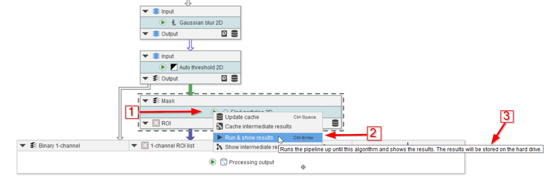
The next option in the menu (red arrow 1) is Run & show results (red arrow 2) that will calculate and save the results as explained on the UI (red arrow 3).
Update cache and Cache intermediate results store the results into the RAM, while Run & show results amd Show intermediate results store all results to the hard drive into a temporary directory (also see the tutorial how to change this directory). Each option has different benefits and disadvantages:
- Caching to RAM:
- Benefit: Fast, convenient to use, can be updated in-place (for testing parameters)
- Disadvantage: RAM space is limited
- Saving to HDD:
- Benefit: Lower RAM usage
- Disadvantage: Slow due to file loading process, some convenience-features not available
Step 5
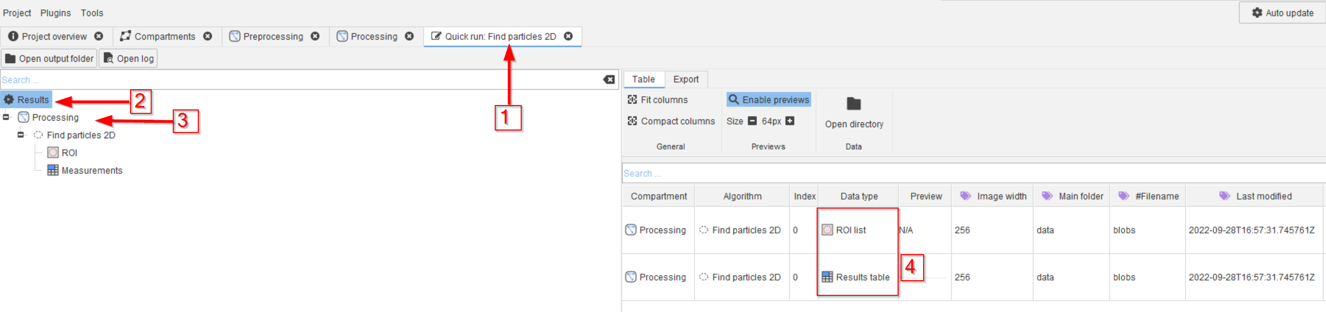
The results will appear in a new tab (red arrow 1) that will present the results (red arrow 2) that will show the origin of the outcome (red arrow 3) as Processing compartment and Find particles 2D node.
The outcome will contain the ROI table and the measurements, as expected for this node (red rectangle 4).
The opened UI is connected to a directory on the hard-drive that is located within the temporary directory as defined by your operating system (also see the tutorial how to change this directory). Opening a data item (double-click) will invoke the loading process and display the data within JIPipe.
Step 6
The last menu (red arrow 1) item Show intermediate results (red arrow 2) performs similarly to the previous option (Run & show results), but presents the results of the intermediate nodes as well as explained by the pop-up comment (red arrow 3, red line 4).
Step 7
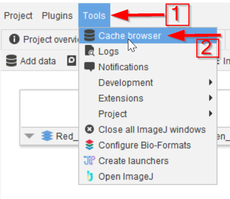
The entire project-wide cache can be viewed and managed via the Tools menu (red arrow 1), using the Cache browser option (red arrow 2).
So far, we only used the Cache browser tab that is associated to a specific node. The global Cache browser option is useful for browsing through all data that has been cached.
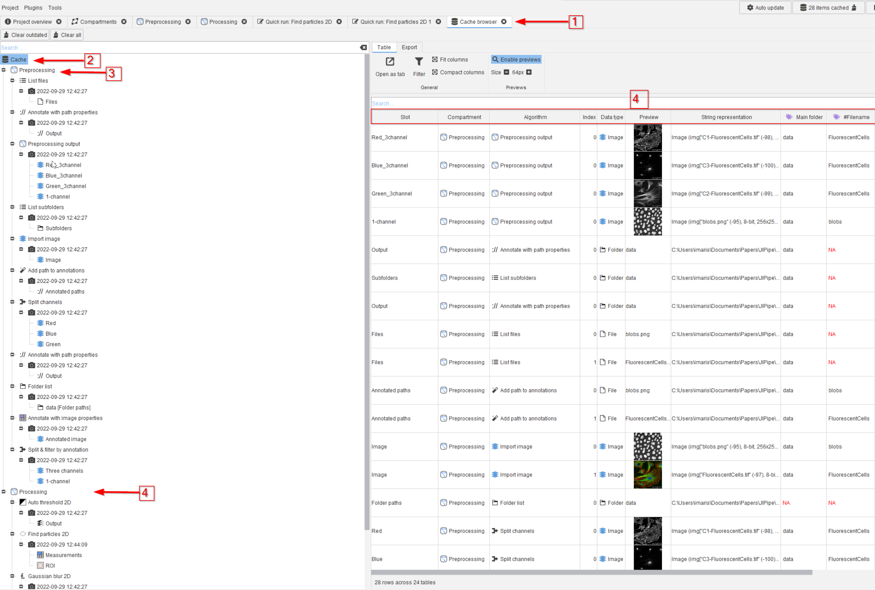
Step 8
The cache browser will open in a new tab of the UI (red arrow 1), where the hierarchy of compartments, nodes, and outputs (red arrow 2 and 3) will appear on the left side. For example, you might also find the outputs of the Processing compartment (red arrow 4).
The cache content appears on the right side of the UI, containing all the results arranged in columns (red rectangle 4).